Working with data in R

Fundamentals of Data Science

Author

Jeremy Teitelbaum

Working with Data in R

load the required libraries

library(tidyverse)
── Attaching core tidyverse packages ──────────────────────── tidyverse 2.0.0 ──
✔ dplyr     1.1.3     ✔ readr     2.1.4
✔ forcats   1.0.0     ✔ stringr   1.5.0
✔ ggplot2   3.4.2     ✔ tibble    3.2.1
✔ lubridate 1.9.2     ✔ tidyr     1.3.0
✔ purrr     1.0.2     
── Conflicts ────────────────────────────────────────── tidyverse_conflicts() ──
✖ dplyr::filter() masks stats::filter()
✖ dplyr::lag()    masks stats::lag()
ℹ Use the conflicted package (<http://conflicted.r-lib.org/>) to force all conflicts to become errors
library(palmerpenguins)
cat(paste(R.version$version.string, "\n"))
R version 4.3.2 (2023-10-31) 

read the penguins data from a csv file

penguins <- read_csv("data/penguins-raw.csv")
Rows: 344 Columns: 17
── Column specification ────────────────────────────────────────────────────────
Delimiter: ","
chr  (9): studyName, Species, Region, Island, Stage, Individual ID, Clutch C...
dbl  (7): Sample Number, Culmen Length (mm), Culmen Depth (mm), Flipper Leng...
date (1): Date Egg

ℹ Use `spec()` to retrieve the full column specification for this data.
ℹ Specify the column types or set `show_col_types = FALSE` to quiet this message.

select a subset of columns

simpler <- penguins |> select(`Species`, `Body Mass (g)`, `Flipper Length (mm)`)
head(simpler)
# A tibble: 6 × 3
  Species                             `Body Mass (g)` `Flipper Length (mm)`
  <chr>                                         <dbl>                 <dbl>
1 Adelie Penguin (Pygoscelis adeliae)            3750                   181
2 Adelie Penguin (Pygoscelis adeliae)            3800                   186
3 Adelie Penguin (Pygoscelis adeliae)            3250                   195
4 Adelie Penguin (Pygoscelis adeliae)              NA                    NA
5 Adelie Penguin (Pygoscelis adeliae)            3450                   193
6 Adelie Penguin (Pygoscelis adeliae)            3650                   190

count the number of occurrences of each value in the “Island” column

penguins |> count(Island)
# A tibble: 3 × 2
  Island        n
  <chr>     <int>
1 Biscoe      168
2 Dream       124
3 Torgersen    52

count the number of occurrences of each value in the “Species” column

penguins |> count(Species)
# A tibble: 3 × 2
  Species                                       n
  <chr>                                     <int>
1 Adelie Penguin (Pygoscelis adeliae)         152
2 Chinstrap penguin (Pygoscelis antarctica)    68
3 Gentoo penguin (Pygoscelis papua)           124

filter the data to keep only rows where “Sex” is “FEMALE”

females <- penguins |> filter(Sex == "FEMALE")
head(females)
# A tibble: 6 × 17
  studyName `Sample Number` Species          Region Island Stage `Individual ID`
  <chr>               <dbl> <chr>            <chr>  <chr>  <chr> <chr>          
1 PAL0708                 2 Adelie Penguin … Anvers Torge… Adul… N1A2           
2 PAL0708                 3 Adelie Penguin … Anvers Torge… Adul… N2A1           
3 PAL0708                 5 Adelie Penguin … Anvers Torge… Adul… N3A1           
4 PAL0708                 7 Adelie Penguin … Anvers Torge… Adul… N4A1           
5 PAL0708                13 Adelie Penguin … Anvers Torge… Adul… N7A1           
6 PAL0708                16 Adelie Penguin … Anvers Torge… Adul… N8A2           
# ℹ 10 more variables: `Clutch Completion` <chr>, `Date Egg` <date>,
#   `Culmen Length (mm)` <dbl>, `Culmen Depth (mm)` <dbl>,
#   `Flipper Length (mm)` <dbl>, `Body Mass (g)` <dbl>, Sex <chr>,
#   `Delta 15 N (o/oo)` <dbl>, `Delta 13 C (o/oo)` <dbl>, Comments <chr>

filter the data to keep only rows where “Flipper Length (mm)” is greater than “Body Mass (g)” divided by 20

penguins |> filter(`Flipper Length (mm)` > `Body Mass (g)` / 20)
# A tibble: 147 × 17
   studyName `Sample Number` Species         Region Island Stage `Individual ID`
   <chr>               <dbl> <chr>           <chr>  <chr>  <chr> <chr>          
 1 PAL0708                 3 Adelie Penguin… Anvers Torge… Adul… N2A1           
 2 PAL0708                 5 Adelie Penguin… Anvers Torge… Adul… N3A1           
 3 PAL0708                 6 Adelie Penguin… Anvers Torge… Adul… N3A2           
 4 PAL0708                 9 Adelie Penguin… Anvers Torge… Adul… N5A1           
 5 PAL0708                11 Adelie Penguin… Anvers Torge… Adul… N6A1           
 6 PAL0708                13 Adelie Penguin… Anvers Torge… Adul… N7A1           
 7 PAL0708                14 Adelie Penguin… Anvers Torge… Adul… N7A2           
 8 PAL0708                17 Adelie Penguin… Anvers Torge… Adul… N9A1           
 9 PAL0708                19 Adelie Penguin… Anvers Torge… Adul… N10A1          
10 PAL0708                21 Adelie Penguin… Anvers Biscoe Adul… N11A1          
# ℹ 137 more rows
# ℹ 10 more variables: `Clutch Completion` <chr>, `Date Egg` <date>,
#   `Culmen Length (mm)` <dbl>, `Culmen Depth (mm)` <dbl>,
#   `Flipper Length (mm)` <dbl>, `Body Mass (g)` <dbl>, Sex <chr>,
#   `Delta 15 N (o/oo)` <dbl>, `Delta 13 C (o/oo)` <dbl>, Comments <chr>

count the number of missing values in each column

colSums(is.na(penguins))
          studyName       Sample Number             Species              Region 
                  0                   0                   0                   0 
             Island               Stage       Individual ID   Clutch Completion 
                  0                   0                   0                   0 
           Date Egg  Culmen Length (mm)   Culmen Depth (mm) Flipper Length (mm) 
                  0                   2                   2                   2 
      Body Mass (g)                 Sex   Delta 15 N (o/oo)   Delta 13 C (o/oo) 
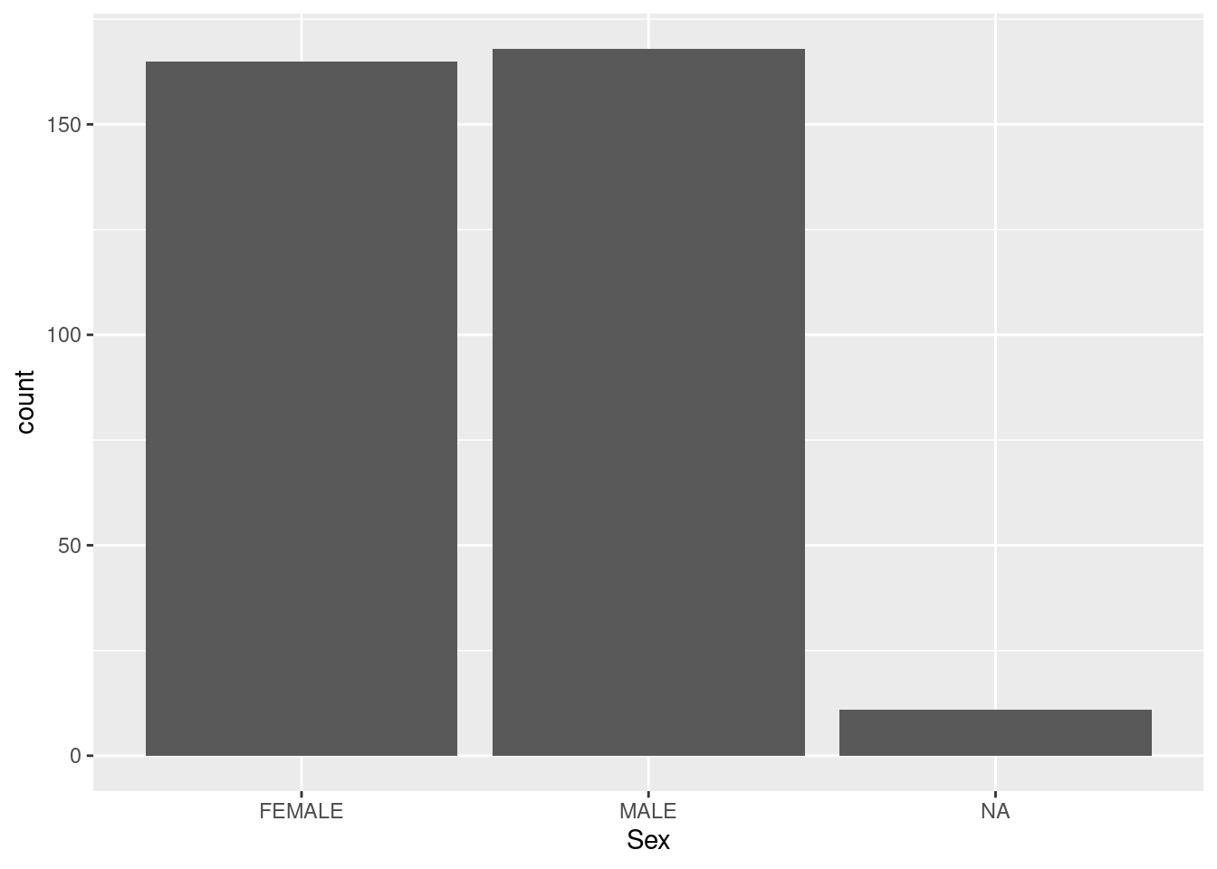
                  2                  11                  14                  13 
           Comments 
                290 

drop the “Comments” column

penguins <- penguins |> select(-Comments)

drop rows with missing values

penguins_nona <- penguins |> drop_na()
dim(penguins_nona)
[1] 324  16

impute missing values in the “Culmen Length (mm)” column with the mean value

penguins_imputed <- penguins |>
    mutate(`Culmen Length (mm)` = if_else(is.na(`Culmen Length (mm)`), mean(`Culmen Length (mm)`, na.rm = TRUE), `Culmen Length (mm)`))

set the “Sex” column as a categorical variable

penguins <- penguins |> mutate(Sex = as.factor(Sex))

Use this factor to get a plot of the number of each sex

ggplot(data = penguins, aes(x = Sex)) +
    geom_bar()

create a new column “SimpleSpecies” by extracting the first word from the “Species” column

penguins <- penguins |> mutate(SimpleSpecies = word(Species, 1))

create a new column “Body Mass (kg)” by dividing the “Body Mass (g)” column by 1000

penguins <- penguins |> mutate(`Body Mass (kg)` = `Body Mass (g)` / 1000)

sort the data by “Body Mass (g)” in ascending order

penguins_small <- penguins |> select(Species, Island, `Body Mass (g)`)
penguins_small |> arrange(`Body Mass (g)`)
# A tibble: 344 × 3
   Species                                   Island    `Body Mass (g)`
   <chr>                                     <chr>               <dbl>
 1 Chinstrap penguin (Pygoscelis antarctica) Dream                2700
 2 Adelie Penguin (Pygoscelis adeliae)       Biscoe               2850
 3 Adelie Penguin (Pygoscelis adeliae)       Biscoe               2850
 4 Adelie Penguin (Pygoscelis adeliae)       Biscoe               2900
 5 Adelie Penguin (Pygoscelis adeliae)       Dream                2900
 6 Adelie Penguin (Pygoscelis adeliae)       Torgersen            2900
 7 Chinstrap penguin (Pygoscelis antarctica) Dream                2900
 8 Adelie Penguin (Pygoscelis adeliae)       Biscoe               2925
 9 Adelie Penguin (Pygoscelis adeliae)       Dream                2975
10 Adelie Penguin (Pygoscelis adeliae)       Dream                3000
# ℹ 334 more rows

group the data by “Species”

penguins_by_species <- penguins |> group_by(Species)
#### summarize the "Body Mass (g)" column for each group
penguins_by_species |> drop_na()|> summarize(mean = mean(`Body Mass (g)`), sd = sd(`Body Mass (g)`), n = n())
# A tibble: 3 × 4
  Species                                    mean    sd     n
  <chr>                                     <dbl> <dbl> <int>
1 Adelie Penguin (Pygoscelis adeliae)       3703.  460.   139
2 Chinstrap penguin (Pygoscelis antarctica) 3730.  386.    67
3 Gentoo penguin (Pygoscelis papua)         5091.  503.   118

group the data by “Sex” and “Species”

penguins_by_sex_and_species <- penguins |> group_by(Sex, Species)

summarize the “Body Mass (g)” column for each group

penguins_by_sex_and_species |> summarize(mean = mean(`Body Mass (g)`), sd = sd(`Body Mass (g)`), n = n())
`summarise()` has grouped output by 'Sex'. You can override using the `.groups`
argument.
# A tibble: 8 × 5
# Groups:   Sex [3]
  Sex    Species                                    mean    sd     n
  <fct>  <chr>                                     <dbl> <dbl> <int>
1 FEMALE Adelie Penguin (Pygoscelis adeliae)       3369.  269.    73
2 FEMALE Chinstrap penguin (Pygoscelis antarctica) 3527.  285.    34
3 FEMALE Gentoo penguin (Pygoscelis papua)         4680.  282.    58
4 MALE   Adelie Penguin (Pygoscelis adeliae)       4043.  347.    73
5 MALE   Chinstrap penguin (Pygoscelis antarctica) 3939.  362.    34
6 MALE   Gentoo penguin (Pygoscelis papua)         5485.  313.    61
7 <NA>   Adelie Penguin (Pygoscelis adeliae)         NA    NA      6
8 <NA>   Gentoo penguin (Pygoscelis papua)           NA    NA      5

create a pivot table of the mean “Body Mass (g)” for each combination of “Sex” and “Species”

penguins_by_sex_and_species |>
    summarize(mean = mean(`Body Mass (g)`)) |>
    pivot_wider(names_from = Species, values_from = mean)
`summarise()` has grouped output by 'Sex'. You can override using the `.groups`
argument.
# A tibble: 3 × 4
# Groups:   Sex [3]
  Sex    Adelie Penguin (Pygosce…¹ Chinstrap penguin (P…² Gentoo penguin (Pygo…³
  <fct>                      <dbl>                  <dbl>                  <dbl>
1 FEMALE                     3369.                  3527.                  4680.
2 MALE                       4043.                  3939.                  5485.
3 <NA>                         NA                     NA                     NA 
# ℹ abbreviated names: ¹​`Adelie Penguin (Pygoscelis adeliae)`,
#   ²​`Chinstrap penguin (Pygoscelis antarctica)`,
#   ³​`Gentoo penguin (Pygoscelis papua)`

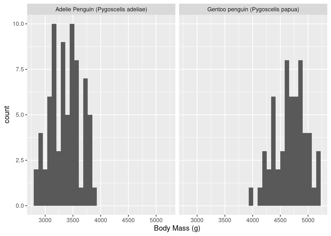
plot a histogram of “Body Mass (g)” for female Adelie and Gentoo penguins

penguins |>
    filter(Species %in% c("Adelie Penguin (Pygoscelis adeliae)", "Gentoo penguin (Pygoscelis papua)"), Sex == "FEMALE") |>
    ggplot(aes(x = `Body Mass (g)`)) +
    geom_histogram(bins = 30) +
    facet_wrap(~Species)

penguins |>
    filter(Species %in% c("Adelie Penguin (Pygoscelis adeliae)", "Gentoo penguin (Pygoscelis papua)"), Sex == "FEMALE") |>
    ggplot(aes(x = `Body Mass (g)`)) +
    geom_histogram(bins = 30) +
    facet_wrap(~Species)

excel files

One can also work with excel files. You need the readxl library.

library("readxl")

As an example, we use an excel spreadsheet violent crime data from the FBI.

read the 2019 crime data, and remove D.C.

ViolentCrime2019 <-
    read_excel("data/Violent Crime-by state-2019-table-5.xls",
        sheet = 1, range = "A4:M514", trim_ws = TRUE
    )
New names:
• `` -> `...3`
ViolentCrime2019
# A tibble: 510 × 13
   State  Area  ...3  Population `Violent \ncrime1` Murder and \nnonnegl…¹ Rape2
   <chr>  <chr> <chr> <chr>                   <dbl>                  <dbl> <dbl>
 1 ALABA… Metr… <NA>  3728978                    NA                     NA    NA
 2 <NA>   <NA>  Area… 0.7660000…              12880                    182  1141
 3 <NA>   <NA>  Esti… 1                       19951                    300  1542
 4 <NA>   Citi… <NA>  528518                     NA                     NA    NA
 5 <NA>   <NA>  Area… 0.8930000…               3327                     36   297
 6 <NA>   <NA>  Esti… 1                        3541                     37   310
 7 <NA>   Nonm… <NA>  645689                     NA                     NA    NA
 8 <NA>   <NA>  Area… 0.7239999…                874                     13   148
 9 <NA>   <NA>  Esti… 1                        1554                     21   216
10 <NA>   Stat… <NA>  4903185                 25046                    358  2068
# ℹ 500 more rows
# ℹ abbreviated name: ¹​`Murder and \nnonnegligent \nmanslaughter`
# ℹ 6 more variables: Robbery <dbl>, `Aggravated \nassault` <dbl>,
#   `Property \ncrime` <dbl>, Burglary <dbl>, `Larceny-theft` <dbl>,
#   `Motor \nvehicle \ntheft` <dbl>

Notice that the third column got a “made-up” name (‘..3’) and the other column names are a bit weird, they have newlines in them and also in some case footnotes. Let’s clean this up. First we replace all of the newlines and spaces by underlines in the column names.

colnames(ViolentCrime2019) = gsub("[ \n]+", "_", colnames(ViolentCrime2019))
ViolentCrime2019
# A tibble: 510 × 13
   State   Area     ...3  Population Violent_crime1 Murder_and_nonneglig…¹ Rape2
   <chr>   <chr>    <chr> <chr>               <dbl>                  <dbl> <dbl>
 1 ALABAMA Metropo… <NA>  3728978                NA                     NA    NA
 2 <NA>    <NA>     Area… 0.7660000…          12880                    182  1141
 3 <NA>    <NA>     Esti… 1                   19951                    300  1542
 4 <NA>    Cities … <NA>  528518                 NA                     NA    NA
 5 <NA>    <NA>     Area… 0.8930000…           3327                     36   297
 6 <NA>    <NA>     Esti… 1                    3541                     37   310
 7 <NA>    Nonmetr… <NA>  645689                 NA                     NA    NA
 8 <NA>    <NA>     Area… 0.7239999…            874                     13   148
 9 <NA>    <NA>     Esti… 1                    1554                     21   216
10 <NA>    State T… <NA>  4903185             25046                    358  2068
# ℹ 500 more rows
# ℹ abbreviated name: ¹​Murder_and_nonnegligent_manslaughter
# ℹ 6 more variables: Robbery <dbl>, Aggravated_assault <dbl>,
#   Property_crime <dbl>, Burglary <dbl>, `Larceny-theft` <dbl>,
#   Motor_vehicle_theft <dbl>

Next we pull out the names from taking the state column, omitting the “NA” values, and treating this as strings. We also want a list for later work, not a tibble.

States <- ViolentCrime2019 |>
    select("State") |>
    drop_na()
States = States$State
States
 [1] "ALABAMA"               "ALASKA"                "ARIZONA"              
 [4] "ARKANSAS"              "CALIFORNIA"            "COLORADO"             
 [7] "CONNECTICUT"           "DELAWARE"              "DISTRICT OF COLUMBIA3"
[10] "FLORIDA"               "GEORGIA"               "HAWAII"               
[13] "IDAHO"                 "ILLINOIS"              "INDIANA"              
[16] "IOWA"                  "KANSAS"                "KENTUCKY"             
[19] "LOUISIANA"             "MAINE"                 "MARYLAND"             
[22] "MASSACHUSETTS"         "MICHIGAN"              "MINNESOTA"            
[25] "MISSISSIPPI4"          "MISSOURI"              "MONTANA"              
[28] "NEBRASKA"              "NEVADA"                "NEW HAMPSHIRE"        
[31] "NEW JERSEY"            "NEW MEXICO"            "NEW YORK"             
[34] "NORTH CAROLINA"        "NORTH DAKOTA"          "OHIO4"                
[37] "OKLAHOMA"              "OREGON4"               "PENNSYLVANIA"         
[40] "PUERTO RICO"           "RHODE ISLAND"          "SOUTH CAROLINA"       
[43] "SOUTH DAKOTA"          "TENNESSEE"             "TEXAS"                
[46] "UTAH"                  "VERMONT"               "VIRGINIA"             
[49] "WASHINGTON"            "WEST VIRGINIA"         "WISCONSIN"            
[52] "WYOMING"              

State number 9 is DC and state number 40 is Puerto Rico. We can drop those.

States <- States[c(-9, -40)]
States
 [1] "ALABAMA"        "ALASKA"         "ARIZONA"        "ARKANSAS"      
 [5] "CALIFORNIA"     "COLORADO"       "CONNECTICUT"    "DELAWARE"      
 [9] "FLORIDA"        "GEORGIA"        "HAWAII"         "IDAHO"         
[13] "ILLINOIS"       "INDIANA"        "IOWA"           "KANSAS"        
[17] "KENTUCKY"       "LOUISIANA"      "MAINE"          "MARYLAND"      
[21] "MASSACHUSETTS"  "MICHIGAN"       "MINNESOTA"      "MISSISSIPPI4"  
[25] "MISSOURI"       "MONTANA"        "NEBRASKA"       "NEVADA"        
[29] "NEW HAMPSHIRE"  "NEW JERSEY"     "NEW MEXICO"     "NEW YORK"      
[33] "NORTH CAROLINA" "NORTH DAKOTA"   "OHIO4"          "OKLAHOMA"      
[37] "OREGON4"        "PENNSYLVANIA"   "RHODE ISLAND"   "SOUTH CAROLINA"
[41] "SOUTH DAKOTA"   "TENNESSEE"      "TEXAS"          "UTAH"          
[45] "VERMONT"        "VIRGINIA"       "WASHINGTON"     "WEST VIRGINIA" 
[49] "WISCONSIN"      "WYOMING"       

Finally, suppose we’re only interested in the state totals. That means which need to extract the rows where the “Area” column is “State Total”.

 VCrimeRate2019 <- ViolentCrime2019 |>
     filter(`Area` == "State Total") |>
     select(`Violent_crime1`)
 VCrimeRate2019
# A tibble: 50 × 1
   Violent_crime1
            <dbl>
 1          25046
 2           6343
 3          33141
 4          17643
 5         174331
 6          21938
 7           6546
 8           4115
 9          81270
10          36170
# ℹ 40 more rows