R Notebook Walkthrough

Fundamentals of Data Science

Author

Jeremy Teitelbaum

Start out with a code cell saying “Hello World”

print("Hello World")

[1] "Hello World"

The cat command is actually probably more useful than print:

cat("hello world")

hello world

Variables, Types, and Assignment

In R, the assignment operator is <-, not =. This takes some getting used to.

count <- 5
name <- "Jeremy Teitelbaum" # string types are called chr for character
paragraph <- "Far across the misty mountains cold,
to dungeons deep and caverns cold,
we must away,
ere break of day
to seek our long forgotten gold."
pi <- 3.14159 # R doesn't use integer types unless you force it to, numbers are "num" # nolint: line_length_linter.
epsilon <- 1e-6
count <- 5L # this forces an integer
students <- c("Jeremy", "Phillip", "Sara", "Molly")
hot_dog <- TRUE # note all caps unlike Python; false is FALSE

In R, you can give names to the elements of a vector.

print("hello")

[1] "hello"

names(students) <- c("President", "Vice President", "Treasurer", "Secretary")
print(names(students))

[1] "President"      "Vice President" "Treasurer"      "Secretary"

print(students["President"])

President 
 "Jeremy"

print(students)

     President Vice President      Treasurer      Secretary 
      "Jeremy"      "Phillip"         "Sara"        "Molly"

The cat command is a print command that “concatenates” its arguments; it needs an explicit newline.

print(students)

     President Vice President      Treasurer      Secretary 
      "Jeremy"      "Phillip"         "Sara"        "Molly"

print(count)

[1] 5

cat("Students:", students, "\n")

Students: Jeremy Phillip Sara Molly

print(epsilon)

[1] 1e-06

cat("The value of epsilon is:", epsilon, "\n")

The value of epsilon is: 1e-06

print(paragraph)

[1] "Far across the misty mountains cold,\nto dungeons deep and caverns cold,\nwe must away,\nere break of day\nto seek our long forgotten gold."

cat(paragraph)

Far across the misty mountains cold,
to dungeons deep and caverns cold,
we must away,
ere break of day
to seek our long forgotten gold.

The [1] at the beginning of each of these things reflects the fact that in R everything is a vector. So it is telling you that the first thing there is element 1 of the vector.

The c() command makes a vector of its arguments. It forces everything to be of the same type.

str_list <- c("Jeremy", 25, 1.34, FALSE) # everything becomes a string
int_list <- c(1, 2, 3, 4, 5)
float_list <- c(1, 2, 3.5, 4)

Arithmetic

R does all arithmetic on vectors/lists. It one is shorter than the other, it repeats the shorter one, but the length of the longer has to be a multiple of the shorter.

a <- 1
b <- 2
a + b

[1] 3

a <- c(1, 2, 3, 4, 5)
b <- 4
a + b

[1] 5 6 7 8 9

a <- c(1, 2, 3, 4, 5, 6)
b <- c(10, 11)
a + b

[1] 11 13 13 15 15 17

a <- c(1, 2, 3, 4, 5)
b <- c(1, 2)
a + b

Warning in a + b: longer object length is not a multiple of shorter object
length

[1] 2 4 4 6 6

a / 5

[1] 0.2 0.4 0.6 0.8 1.0

# integer division (// in python)
a <- 5L
b <- 3
a %/% b

[1] 1

# remainder (% in python)
a <- 5
b <- 3
a %% b

[1] 2

a <- c(1, 2, 3, 4, 5)
a^2

[1]  1  4  9 16 25

print(a^2 == a)

[1]  TRUE FALSE FALSE FALSE FALSE

print(a^2 > a)

[1] FALSE  TRUE  TRUE  TRUE  TRUE

print(a^2 == 4)

[1] FALSE  TRUE FALSE FALSE FALSE

Operations on strings and lists

first_name <- "Jeremy"
last_name <- "Teitelbaum"
nchar(first_name)

[1] 6

paste(first_name, last_name) # spaces by default

[1] "Jeremy Teitelbaum"

paste(first_name, last_name, sep = "") # no space

[1] "JeremyTeitelbaum"

paste(c(1, 2, 3), "Jeremy") # remember functions work across vectors

[1] "1 Jeremy" "2 Jeremy" "3 Jeremy"

Substrings

In R, you always count from 1 (big difference from python)

first_name[1] # another difference from Python

[1] "Jeremy"

a <- substr("Jeremy", 1, 1)
b <- substr("Jeremy", 1, 3)
cat(a, b, paste(a, b, sep = ""))

J Jer JJer

Slicing lists

nums <- 0:10 # generates a sequence from 0 to 10 INCLUSIVE (compare python)
print(nums)

 [1]  0  1  2  3  4  5  6  7  8  9 10

print(nums[c(1, 3)]) # you can pass a list of indices to a subscript

[1] 0 2

sqrs <- nums^2
sqrs[seq(1, 10, 2)]

[1]  0  4 16 36 64

In R, negative numbers in seq mean “omit” so this means omit entries 2 through 5. You can’t mix positive and negative numbers

rev <- nums[seq(-2, -5)]
print(rev)

[1]  0  5  6  7  8  9 10

rev(nums) # reverses the list

 [1] 10  9  8  7  6  5  4  3  2  1  0

Libraries and packages

Use the Rstudio package manager to add libraries to your installation, but to use them you need to use the library function. The tidyverse library is something we will use a lot.

library(tidyverse)

── Attaching core tidyverse packages ──────────────────────── tidyverse 2.0.0 ──
✔ dplyr     1.1.3     ✔ readr     2.1.4
✔ forcats   1.0.0     ✔ stringr   1.5.0
✔ ggplot2   3.4.2     ✔ tibble    3.2.1
✔ lubridate 1.9.2     ✔ tidyr     1.3.0
✔ purrr     1.0.2     
── Conflicts ────────────────────────────────────────── tidyverse_conflicts() ──
✖ dplyr::filter() masks stats::filter()
✖ dplyr::lag()    masks stats::lag()
ℹ Use the conflicted package (<http://conflicted.r-lib.org/>) to force all conflicts to become errors

Plotting

library(ggplot2)

x <- seq(-10, 10, .1)
y <- x**2
data <- tibble("x" = x, "y" = y)

ggplot(data = data, aes(x = x)) +
    geom_point(aes(y = y), color = "red") +
    ggtitle("A Parabola") +
    scale_x_continuous(breaks = seq(-10, 10, 1)) +
    scale_y_continuous(breaks = seq(0, 100, 20))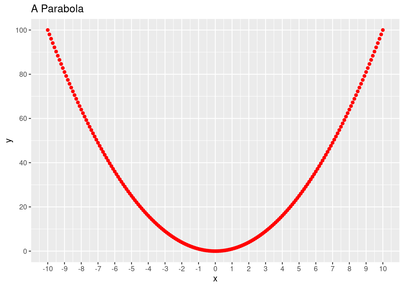

x <- seq(-10, 10, .1)
y <- cos(x)
data <- tibble("x" = x, "y" = y)
ggplot(data = data, aes(x = x)) +
    geom_line(aes(y = y), color = "darkgreen") +
    ggtitle("A Cosine Curve") +
    scale_x_continuous(breaks = seq(-10, 10, 1)) +
    scale_y_continuous(breaks = seq(-1, 1, 5))