Bayesian Online Changepoint Detection
import numpy as np
import matplotlib.pyplot as plt
from scipy.stats import poisson
Introduction
Suppose that we have a sequence of data $x_1, x_2, \ldots, x_N$ produced by some statistical process, such as a poisson process. Imagine that the rate of that process from $i=1$ to $K$ is $\lambda_1=1$, and that for some reason the rate changes abruptly to $\lambda=5$.
data = np.concatenate((poisson(1).rvs(100),poisson(5).rvs(100)))
ax=plt.plot(np.array(range(200)),data,color='gray')
ax=plt.vlines(x=100,ymin=1,ymax=5,linewidth=3,color='red')
ax=plt.hlines([1,5],[0,100],[100,200],linewidth=3,color='red')
ax=plt.title('Changepoint occurs at t=100')
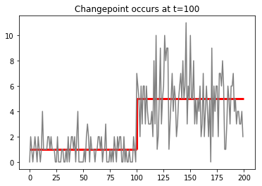
For example, these data could be counts of reads in bins along a chromosome coming from a low-coverage whole genome sequencing experiment done to detect copy number variation.
We would like to identify the transition point, or changepoint, in the data in order to detect regions where there is a copy-number change.
Of course, a similar problem might occur with other sequential data, such as a time series of stock prices, where we are interested in points where a substantive change has occured in the mean price of the stock over time.
The paper Bayesian Online Changepoint Detection describes an algorithm for locating such points. The algorithm uses bayesian reasoning, and it is online in the sense that it operates by reading one data point at a time and providing estimates of the likelihood of a changepoint at a given time based only on information up to that point in time.
The approach taken in this paper is to imagine that the data appears in intervals, or runs, $x_1,\ldots, x_r$ and that within each run the results are i.i.d. At a changepoint, the distribution changes and a yields a new sequence of i.i.d variables from that distribution. The length of the run is a random variable, and the distributions within a run are assumed to come from a single exponential family. For example, the distributions might be normal (with mean and variance changing at the transition points) or poisson (with the rate changing at the transition point as in the example above.)
The idea behind the algorithm is that, as we read a new datum, either that datum comes from the same distribution and the length of the run goes up by one; or that datum represents a change point, in which case the run length resets to zero. If the run length goes up by one, the new datum provides information to improve our estimate of the parameters of the current distribution using Bayes theorem; or, if the run length resets to zero, then we set the distribution back to a pre-chosen initial distribution and begin updating its parameters based on the new datum.
Algorithm Steps
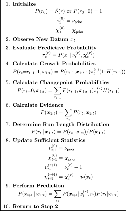
Let’s walk through the steps in the algorithm, referring to the table above taken from the paper.
First notice that $r_t$, the run-length, is a stochastic process on the integers – so that $r_m(n)$ is the probability that the run length at time $m$ is $n$.
Let’s also assume that the distribution that generates our sequence of $x$ has hyperparamenters $\chi$. Again, $\chi_t(r)$ is the value of the hyperparameters at time $t$ if the run length is $r$.
We have $\chi_{t}(0)=\chi$ for all $t$. This means that, if the run length is zero, our distribution generating the data has pre-assigned hyperparameters $\chi$.
Finally, let’s assume that the ‘natural chance’ of a changepoint is $1/\lambda$ – so the mean length of a segment will be $\lambda$ in the absence of any other information. In other words, $P(r_{t+1}=m|r_{t}=n)$ is zero except in these two cases:
For the sake of simplicity, let’s initialize the data so that $r_{0}(0)=1$ and $r_{0}(x)=0$ if $x>1$. This means that our process starts off at $t=0$ with run length zero and the hyperparameters $\chi_{1}(0)$ set to their ‘prior’ values.
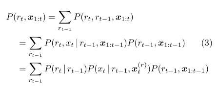
Imagine now that the algorithm has been running up to time $t-1$. This means that we have computed $r_{t-1}(n)$, the probability of run lengths $n=0,\ldots, t-1$ at time $t$. For each such run length, we have also computed hyperparameters of our distribution $\chi_{t}(n)$ for $n=0,\ldots, t$. In other words, we know the total probability distribution $P(r_{t-1},x_1,\ldots, x_{t-1})$.
Now a new piece of information arrives: $x_t$. How does this influence our understanding of the situation?
Referring back to equation 3 of the paper, we see that we have a recursive way to compute $P(r_t, x_1,\ldots, x_t)$:
In this sum, first we have that $P(r_t|r_{t-1})=0$ unless either $r_t=r_{t-1}+1$ (in which case it is $(1-1/\lambda)$) or $r_t=0$ (in which case it is $1/\lambda$). So for $n>0$ we have that
$P(r_t=n, x_1, \ldots, x_t)$ is the product of three terms:
- $(1-1/\lambda)$
- $P(x_{t} | r_{t-1}=n-1, x_{t-1}, \ldots, x_{t-n+1})$
- $P(r_{t-1}=n-1,x_1,\ldots,x_{t-1}).$
The rightmost term is known by recursion. The middle term is computed from the probability distribution for $x$ using the hyperparameters $\chi_{t}^{n-1}$.
On the other hand,
Next, the algorithm computes the distribution $r_{t}(n)=P(r_{t}=n,x_1,\ldots, x_t)/P(x_1,\ldots,x_t)$ where
The final step is to use the new datum $x_t$ to update our predictive distribution, or in other words to update the hyperparameters.
To give a simple example, suppose that our predictive distribution is a Gamma-Poisson distribution (or a negative binomial distribution). In other words, the Poisson rate is Gamma distributed with hyperparameters $k$ and $\theta$, and the mean and variance of this Gamma distribution are $k\theta$ and $k\theta^2$. The predictive distribution on $x$ is negative binomial with parameters $N=k$ and $p=1/(\theta+1)$.
Our initial hyperparameters are chosen as $k_0$ and $\theta_0$. The poisson rate Standard results on conjugate priors tell us that if $P(\lambda)$ has prior parameters $k, \theta$ than the posterior distribution on $\lambda$ after seeing $x$ has parameters $k+x, \theta/(\theta+1)$.
The predictive distribution on $x$ becomes negative binomial with parameters $N+x$ and $(1+\theta)/(1+2\theta)$.
A very nice implementation of this algorithm is available here, where there is a jupyter notebook that works out an example of this algorithm and also an “offline” algorithm that we don’t discuss. Here is the relevant routine for the offline algorithm.
In the implementation, the matrix R is such that R[m,n] is the probability at time n
that the run length is m. The array maxes is the array of most likely run length at each time.
The implementation here uses a ‘T’-distribution as the prior, which is appropriate for a time series that is normally distributed within intervals. More specifically, it uses a normal distribution with normal-inverse gamma priors on $\mu$ and $\sigma^2$. The updating formulae are available in the wikipedia table for conjugate priors.. The relevant row in the table is here:

The following code for a “Poisson-Gamma” distribution can be used instead for count data.
class Poisson:
def __init__(self, k, theta):
self.k0 = self.k = np.array([k])
self.theta0 = self.theta = np.array([theta])

def pdf(self, data):
return stats.nbinom.pmf(data,self.k, 1/(1+self.theta))

def update_theta(self, data):
kT0 = np.concatenate((self.k0, self.k+data))
thetaT0 = np.concatenate((self.theta0, self.theta/(1+self.theta)))

self.k = kT0
self.theta = thetaT0