Python normalizations of Gamma-Poisson and Negative Binomial Distributions

import numpy as np
import matplotlib.pyplot as plt
from scipy.stats import gamma, poisson, nbinom

The Gamma-Poisson (Negative Binomial) mixture distribution

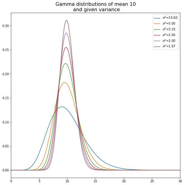
Gamma distributions

fig, ax = plt.subplots(1)
fig.set_size_inches(10,10)
ax.set_xlim([0,30])
G = np.zeros(600000)
G = G.reshape((6,100000))
for i in range(1,7):
g=gamma(10*i,scale = 1.0/i)
G[i-1,:] = g.rvs(100000)
p = ax.plot(np.linspace(0,30,1000),g.pdf(np.linspace(0,30,1000)), label='$\sigma^2$={:.2f}'.format(10.0/i))
p= ax.legend()
p = plt.title('Gamma distributions of mean 10\n and given variance',fontsize=16)

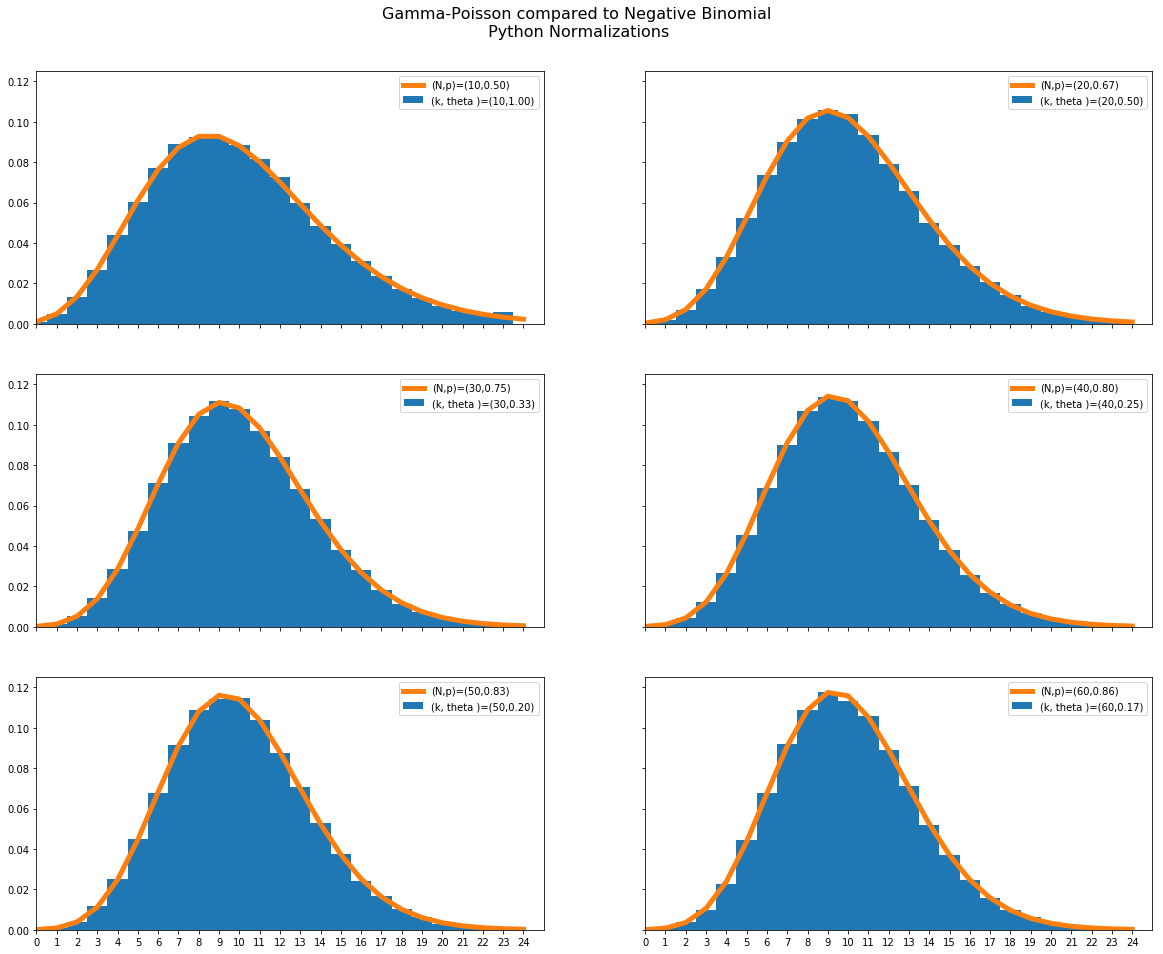
Gamma-Poisson mixtures

If $(k,\theta)$ are the parameters to the gamma function (in python, gamma(k,scale=theta) then the mixture distribution obtained by choosing the poisson rate from this gamma and then choosing a poisson yields a negative binomial with parameters $(N,p)=(k,1/(1+\theta)$ (in python, nbinom(k,1/(1+theta)).

To verify this, we choose random variables in this way and compare with the nbinom pmf in these graphs.

import seaborn as sns
fig, ax = plt.subplots(3,2,sharex=True,sharey=True)
fig.set_size_inches(20,15)
P = poisson(G).rvs()
for i in range(3):
for j in range(2):
ax[i,j].set_xlim([0,25])
plt.xticks(range(25))
ax[i,j].set_ylim([0,.125])
m = 2*i+j+1
ax[i,j].hist(P[2*i+j,:],bins=range(25),density=True,align='left',label='(k, theta )=({},{:.2f})'.format(10*m,1/m))
N = nbinom(10*m,m/(m+1))
ax[i,j].plot(range(25),N.pmf(range(25)),label='(N,p)=({},{:.2f})'.format(10*m, m/(m+1)),linewidth=5)
ax[i,j].legend()
j=fig.suptitle('Gamma-Poisson compared to Negative Binomial\n Python Normalizations',fontsize=16)
fig.subplots_adjust(top=.92)