Gaussian Mixture in Stan

Gaussian Mixture Model via Stan (MCMC)

import pystan
import pandas as pd
import numpy as np
import matplotlib
import matplotlib.pyplot as plt
matplotlib.rcParams['figure.figsize']=10,10
plt.style.use('ggplot')

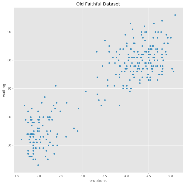
df = pd.read_csv('old_faithful.csv',header=0,index_col=0)
scatter=df.plot.scatter(x='eruptions',y='waiting',title='Old Faithful Dataset')

The stan code and fit

The following stan code was taken from Michael Betancourt’s discussion of degeneracy in mixture models. The thrust of his article is that symmetry among the components of the mixture make it a problem for MCMC sampling. In this code, the means mu are given an “ordered” type which breaks that symmetry by artificially distinguishing between the components.

Note: This handles only one dimension of the data (eruptions).

beta_code="""
data {
 int<lower = 0> N;
 vector[N] y;
}

parameters {
  ordered[2] mu;
  real<lower=0> sigma[2];
  real<lower=0, upper=1> theta;
}

model {
 sigma ~ normal(0, 2);
 mu ~ normal(0, 2);
 theta ~ beta(5, 5);
 for (n in 1:N)
   target += log_mix(theta,
                     normal_lpdf(y[n] | mu[1], sigma[1]),
                     normal_lpdf(y[n] | mu[2], sigma[2]));
}
"""

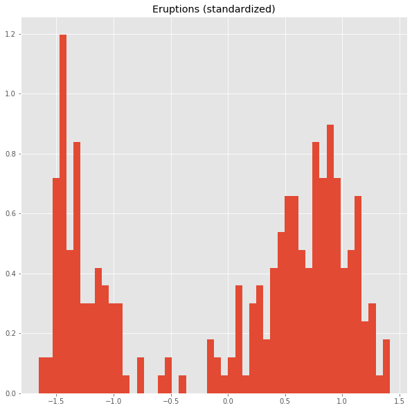
We standardize the data.

from sklearn.preprocessing import StandardScaler
dfs = StandardScaler().fit_transform(df)
plt.title('Eruptions (standardized)')
ax=plt.hist(dfs[:,0],bins=50,density=True)

model = pystan.StanModel(model_code=beta_code)

INFO:pystan:COMPILING THE C++ CODE FOR MODEL anon_model_4a1a8842066ad04ed5bb50ec34a6de05 NOW.

faithful_data={'N':dfs.shape[0],'y':dfs[:,0]}
fit = model.sampling(data=faithful_data,iter=10000,warmup=1000)

The result of the sampling

print(fit)

Inference for Stan model: anon_model_4a1a8842066ad04ed5bb50ec34a6de05.
4 chains, each with iter=10000; warmup=1000; thin=1; 
post-warmup draws per chain=9000, total post-warmup draws=36000.

           mean se_mean     sd   2.5%    25%    50%    75%  97.5%  n_eff   Rhat
mu[1]     -1.29  1.3e-4   0.02  -1.33   -1.3  -1.29  -1.27  -1.24  31364    1.0
mu[2]      0.69  1.4e-4   0.03   0.63   0.67   0.69   0.71   0.75  44695    1.0
sigma[1]   0.21  1.1e-4   0.02   0.18    0.2   0.21   0.23   0.26  33690    1.0
sigma[2]   0.38  1.3e-4   0.02   0.34   0.37   0.38    0.4   0.43  37065    1.0
theta      0.35  1.4e-4   0.03    0.3   0.34   0.35   0.37   0.41  44342    1.0
lp__     -252.9    0.01   1.58 -256.8 -253.7 -252.5 -251.7 -250.8  16745    1.0

Samples were drawn using NUTS at Tue Oct 29 10:22:55 2019.
For each parameter, n_eff is a crude measure of effective sample size,
and Rhat is the potential scale reduction factor on split chains (at 
convergence, Rhat=1).

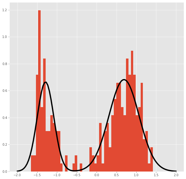
Plot of the distribution obtained from the posterior mean parameters.

from scipy.stats import norm
fig,axes = plt.subplots(1)
axes.hist(dfs[:,0],bins=50,density=True)
x=np.linspace(-2,2,100)
ax=axes.plot(x,.65*norm.pdf(x,loc=.69,scale=.38)+(.35)*norm.pdf(x,loc=-1.29,scale=0.21),linewidth=4,color='black')