Another look at EM

Another look at expectation maximization and gaussian mixtures – long winded!

We will consider the one dimensional case. To make things concrete we will work with the famous “old faithful” dataset.

import pandas as pd
import numpy as np
from scipy.stats import norm
import matplotlib
import matplotlib.pyplot as plt
plt.style.use('seaborn')
matplotlib.rcParams['figure.figsize']=10,10

A look at the data

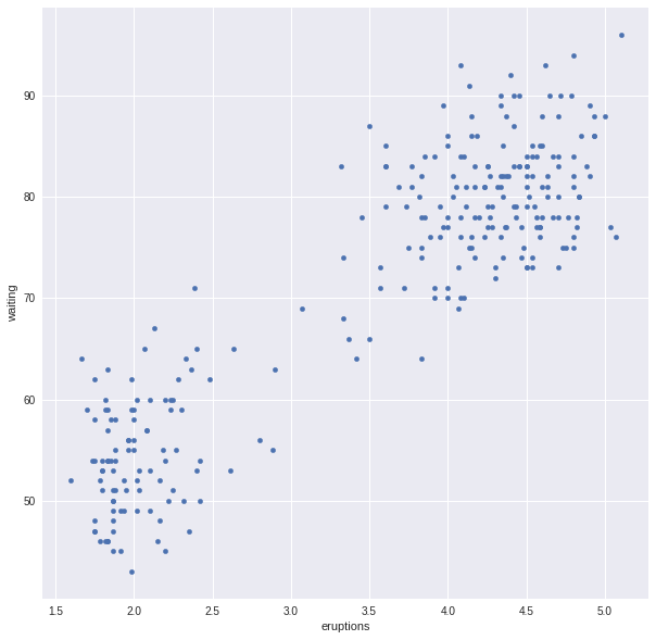
data = pd.read_csv('old_faithful.csv',index_col=0)
ax=data.plot.scatter(x='eruptions',y='waiting')

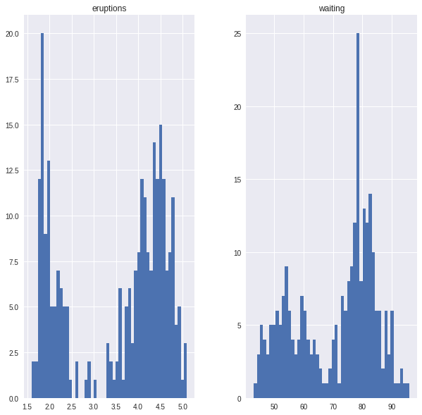
ax=data.hist(bins=50)

The goal is to fit a mixture of two gaussians to (say) the eruptions data. Such a model is given by five parameters:

• $\theta$ is the weight attached to one of the gaussians, $1-\theta$ is the other weight
• $\mu_0,\sigma_0$ are the mean and standard deviation of the first gaussian
• $\mu_1,\sigma_1$ are the mean and standard deviation of the other.

We will use $\mu,\sigma$ to denote the pairs of means and deviations for simplicity.

For future reference, recall that the normal distribution is

$$N(x|\mu,\sigma) = \frac{1}{\sqrt{2\pi\sigma^2}}e^{\frac{(x-\mu)^2}{2\sigma^2}}$$

The distribution function for the mixture is

$$P(x|\theta,\mu,\sigma) = \theta N(x|\mu_0,\sigma_0) + (1-\theta) N(x|\mu_1,\sigma_1)$$

The first step of expectation maximization is to introduce a “latent” or hidden variable $z$ which can take values $0$ or $1$. The events in the expanded model with explicit variables are pairs $(x,0)$ or $(x,1)$ corresponding to whether $x$ arose from one or the other underlying gaussians. Let $p(z)=\theta$ if $z=0$ or $1-\theta$ if $z=1$. Then the joint probability distribution for $(x,z)$ is:

$$P((x,z)|\theta,\mu,\sigma)=\begin{cases} \theta N(x|\mu_0,\sigma_0) & z=0 \cr (1-\theta) N(x|\mu_1,\sigma_1) & z=1\cr \end{cases}$$

The marginal probability of $x$ is the mixture:

$$P(x|\theta,\mu,\sigma) = \sum_z P((x,z)|\theta,\mu,\sigma) = \theta N(x|\mu_0,\sigma_0) + (1-\theta) N(x|\mu_1,\sigma_1)$$

The conditional probabilities are going to be relevant, so let’s look at them. \begin{eqnarray} P(z|x,\theta,\mu,\sigma) &=& \frac{P((x,z)|\theta,\mu,\sigma)}{P(x|\theta,\mu,\sigma)} \cr &=& \frac{p(z)N(x|\mu_z,\sigma_z)}{\sum_z P((x,z)|\theta,\mu,\sigma)} \end{eqnarray}

For the other conditional probability:

$$P(x|z,\theta,\mu,\sigma) = \frac{P((x,z)|\theta,\mu,\sigma)}{P(z|\theta,\mu,\sigma)}$$

which boils down to

$$P(x|z,\theta,\mu,\sigma) = \begin{cases} N(x|\mu_0,\sigma_0) & z=0 \cr N(x|\mu_1,\sigma_1) & z=1 \cr\end{cases}$$

Now let’s go back to the actual data. Expectation maximization is an iterative algorithm that begins with more or less arbitary parameters and then successively improves them. The goal is to find parameters $\theta,\mu,\sigma$ that make the data most likely. For clarity, we will write $\mathbf{x}$ and $\mathbf{z}$ to be the vector of data points $(x_1,\ldots, x_n)$ and a vector of “assignments” $(z_1,\ldots, z_n)$.

The trick is to consider a probability distribution $q(\mathbf{z})$ on the vector of assignments of each data point to a cluster. For any such distribution we have a tautological result:

\begin{eqnarray} \log P(\mathbf{x}|\theta,\mu,\sigma) &=& \sum_{\mathbf{z}}q(\mathbf{z})\log P(\mathbf{x}|\theta,\mu,\sigma) \cr &=& \sum_{\mathbf{z}}q(\mathbf{z})\log\frac{P(\mathbf{x},\mathbf{z}|\theta,\mu,\sigma)}{P(\mathbf{z}|\mathbf{x},\theta,\mu,\sigma)} \cr \end{eqnarray}

and this can be rearranged to yield

$$P(\mathbf{x}|\theta,\mu,\sigma) = \sum_{\mathbf{z}}q(\mathbf{z})\log\frac{P((\mathbf{x},\mathbf{z})|\theta,\sigma,\mu)}{q(\mathbf{z})} -\sum_{\mathbf{z}}q(\mathbf{z})\log\frac{P(\mathbf{z}|\mathbf{x},\sigma,\mu,\theta)}{q(\mathbf{z})}$$

Each of the two terms on the right have a particular role in the EM algorithm. Let’s given them names.

$$\mathcal{L}(\theta,\mu,\sigma) = \sum_{\mathbf{z}}q(\mathbf{z})\log\frac{P((\mathbf{x},\mathbf{z})|\theta,\mu,\sigma)}{q(\mathbf{z})}$$ $$KL(q||P) = -\sum_{\mathbf{z}}q(\mathbf{z})\log\frac{P(\mathbf{z}|\mathbf{x},\sigma,\mu,\theta)}{q(\mathbf{z})}$$

The $KL$ term is the “Kullblack-Leibler divergence” between the conditional probability on the vector of cluster assignments and the a priori chosen distribution $q(\mathbf{z})$. This divergence has the property that it is always greater than or equal to zero, and it is zero only when $q(\mathbf{z})=P(\mathbf{z}|\mathbf{x},\sigma,\mu,\theta)$. This is where Jensen’s lemma is applied, because the non-negativity of KL is essentially Jensen’s lemma.

The EM strategy works like this. First, we choose $q(\mathbf{z})$ to be $P(\mathbf{z}|\mathbf{x},\sigma,\mu,\theta)$. That forces the KL divergence term to zero. Now we have the log-likelihood of the data equal to $\mathcal{L}$. We can find $\theta’,\mu’,\sigma’$ which maximize $\mathcal{L}$. For those parameters, we have

$$\log P(\mathbf{x}|\theta',\sigma',\mu')=\mathcal{L}(\theta',\mu',\sigma')+KL'>\log P(\mathbf{x}|\theta,\mu,\sigma).$$

The conditional probabilities having changed, the $KL$ term is again non-zero so we can repeat the argument with a new $q$ set to the new conditional probabilities and we can again drive the log-likelihood up.

So the key element here is how to maximize $\mathcal{L}(\theta,\mu,\sigma)$ when

$$q(\mathbf{z})=P(\mathbf{z}|\mathbf{x},\theta,\mu,\sigma).$$

To look at this, first notice that

$$\mathcal{L}(\theta,\mu,\sigma)=\sum_{\mathbf{z}}q(\mathbf{z})\log P((\mathbf{x},\mathbf{z})|\theta,\mu,\sigma)-\sum_{\mathbf{z}}q(\mathbf{z})\log q(\mathbf{z})$$

For the purposes of maximizing $\mathcal{L}$ in this process, $q(\mathbf{z})$ is a constant, so we only need to look at the first term. Using our formulae above, the sum over $\mathbf{z}$ is the sum over all vectors of $1$’s and $0$’s of length $n$, with the probability of a vector given by independent choices with the probability of a zero in the $i^{th}$ position being $P(z=0|x=x_i,\theta,\mu,\sigma)$ which is computed above. In other words, we are summing over all possible assignments of points $x_i$ to one cluster or the other.

In fact we are looking at an expectation over $\mathbf{z}$ of the sum of independent random variables $(x_i,z_i)$ so that result is the sum of the expectationsl

Since for a single pair $(x,z)$ we have

$$\log P((x,z)|\theta,\mu,\sigma)=\begin{cases} \log(\theta)-\log(\sigma_0)-(1/2)\log(2\pi)-\frac{(x-\mu_{0})^2}{2\sigma_0^{2}} & z=0 \cr \log(1-\theta)-\log(\sigma_1)-(1/2)\log(2\pi)-\frac{(x-\mu_1)^2}{2\sigma_1^2} & z=1\cr\end{cases}$$

we have

\begin{eqnarray} E_{z}\log P((x,z)|\theta,\mu,\sigma) &=& [p_z\log(\theta)+(1-p_z)\log(1-\theta)] - [p_z\log(\sigma_0) +(1-p_z)\log(\sigma_1)]\cr && -p_z((x-\mu_0)^2/2\sigma_0^2)-(1-p_z)((x-\mu_1)^2/2\sigma_1^2)+C \end{eqnarray}

Summing this over the coordinates, and taking the relevant derivatives with respect to $\theta$, $\sigma_0$, $\sigma_1$, $\mu_0$ and $\mu_1$ we get the following equations.

Write $q(i)$ for the $i^{th}$ component of the conditional probabilities that were used to construct the distribution $q(\mathbf{z})$:

$$q(i) = P(z=0|x_i,\theta,\mu,\sigma)$$ $$\sum_{i=1}^{n} \frac{q(i)}{\theta}+\frac{1-q(i)}{1-\theta} = 0$$ $$\sum_{i=1}^{n} \frac{q(i)(x_i-\mu_0)}{\sigma_{0}^2}=0$$ $$\sum_{i=1}^{n} -\frac{q(i)}{\sigma_{0}}+\frac{q(i)((x_i-\mu_0)^2)}{\sigma_0^3}=0$$

with two more equations for $\mu_1$ and $\sigma_1$ replacing $q(i)$ with $1-q(i)$.

Let’s let $n_0=\sum_{i=1}^{n} q(i)$ and $n_1=n-n_0$. Then we get the following formulae for the “new” $\theta,\mu,\sigma$:

$$\theta = n_0/n$$ $$\mu_0 = \frac{\sum_{i=1}^{n} q(i)x_i}{n_0}$$ $$\mu_1 = \frac{\sum_{i=1}^{n} (1-q(i))x_i}{n_1}$$ $$\sigma_0^2 = \frac{\sum q(i)(x-\mu_0)^2}{n_0}$$ $$\sigma_1^2 = \frac{\sum (1-q(i))(x-\mu_1)^2}{n_1}$$

Now let’s try this with the data. For initial values, let’s set initial parameters.

x = data['eruptions'].values
theta = 0.5
mu_0, sigma_0 = 2, 1
mu_1, sigma_1 = 4, 1
A = norm(2,1)
B = norm(4,1)

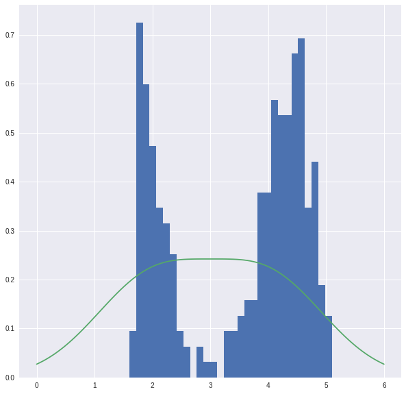
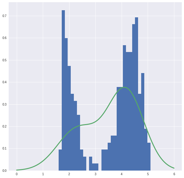
This mixture is not that great, let’s look.

u=np.linspace(0,6,100)
plt.hist(x,density=True,bins=30)
plt.plot(u,theta*A.pdf(u)+(1-theta)*B.pdf(u))

[<matplotlib.lines.Line2D at 0x7ff77b472d10>]

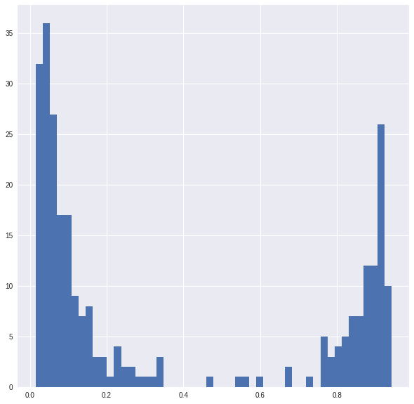
With these parameters, we compute the conditional probabilities that give the distribution $q(\mathbf{z})$.

P = theta*A.pdf(x)/(theta*A.pdf(x)+(1-theta)*B.pdf(x))

P is an estimate of the chance that that a point belongs to one of the two clusters; a quick look shows that P does seem to split the data into two points.

ax=plt.hist(P,bins=50)

Now we can update the parameters according to our formulae.

N = x.shape[0]
N0 = P.sum()
N1 = (1-P).sum()
theta = N0/N
mu0 = (P*x).sum()/N0
mu1 = ((1-P)*x).sum()/N1
sigma0 = np.sqrt(np.sum(P*np.square(x-mu0))/N0)
sigma1 = np.sqrt(np.sum((1-P)*np.square(x-mu1))/N1)

Let’s look at the new mixture.

A = norm(mu0,sigma0)
B = norm(mu1, sigma1)
plt.hist(x,density=True,bins=30)
plt.plot(u,theta*A.pdf(u)+(1-theta)*B.pdf(u),linewidth=3)

[<matplotlib.lines.Line2D at 0x7ff78143b090>]

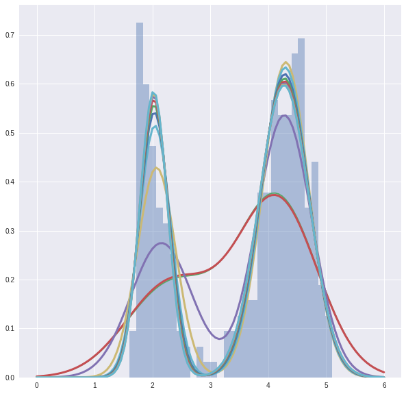
Now we can try to watch the whole process.

plt.hist(x,density=True,bins=30,alpha=.4)
plt.plot(u,theta*A.pdf(u)+(1-theta)*B.pdf(u))
for i in range(10):
    P = theta*A.pdf(x)/(theta*A.pdf(x)+(1-theta)*B.pdf(x))   
    N0 = P.sum()
    N1 = (1-P).sum()
    theta = N0/N
    mu0 = (P*x).sum()/N0
    mu1 = ((1-P)*x).sum()/N1
    sigma0 = np.sqrt(np.sum(P*np.square(x-mu0))/N0)
    sigma1 = np.sqrt(np.sum((1-P)*np.square(x-mu1))/N1)
    plt.plot(u,theta*A.pdf(u)+(1-theta)*B.pdf(u),linewidth=3)
    A = norm(mu0, sigma0)
    B = norm(mu1, sigma1)
    

And the final picture looks like this.

plt.hist(x,density=True,bins=30,alpha=.5)
plt.plot(u,theta*A.pdf(u)+(1-theta)*B.pdf(u),linewidth=4)

[<matplotlib.lines.Line2D at 0x7ff77b1b65d0>]

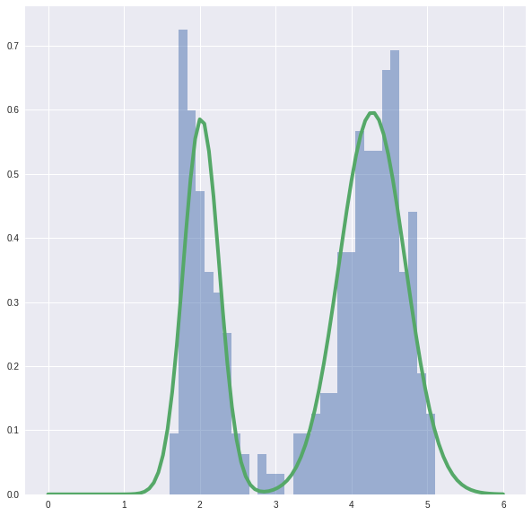
Cool!