GC Bias correction in ginkgo and cnvkit

Correcting for GC bias

import pandas as pd
import numpy as np
import seaborn as sns
from statsmodels.nonparametric.smoothers_lowess import lowess
sns.set_style('darkgrid')

There is a known source of bias in sequencing coming from the relative proportion of GC bases in the sequence in a particular bin. Both ginkgo and cnvkit correct for this bias. We compare their approaches.

We work with the raw counts collected by bedtools coverage for the ginkgo bins as a starting point.

RawCounts=pd.read_table('big.txt')
cells = X.columns[3:]
normal = X.copy()
normal[cells]=normal[cells]/normal[cells].mean()

Ginkgo has already computed the relative proportion of GC bases in its bins and stored it in a file.

GC = pd.read_table('GC_variable_500000_76_bwa',header=None,names=['GC'])

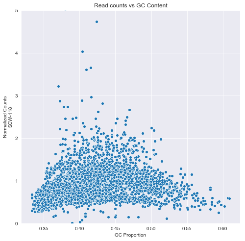
We pick one of the cell samples to illustrate the GC bias. The following scatter plot shows that in bins with higher or lower than balanced GC count, there are fewer counts.

j=sns.scatterplot(GC['GC'],normal[cells].iloc[:,10])
t=j.set_ylim([0,5])
t=j.set_ylabel('Normalized Counts\nSCW-118')
t=j.set_xlabel('GC Proportion')
t=j.set_title('Read counts vs GC Content')
j.get_figure().set_size_inches(8,8)

Local Regression and Ginkgo

Ginkgo compensates for the dependence on GC content by using local regression. Essentially, locally weighted scatterplot smoothing, or LOWESS, applies linear regression to a window of points, weighting the points within the window so that nearer points carry more weight.

This is an ad hoc method for smoothing that has many parameters and variants.

See wikipedia LOWESS for a discussion.

The statsmodels python package implements a version of this. The frac parameter controls the size of the window. Ginkgo uses 0.05.

# computes the corrected value by subtracting off the lowess fit
# for some reason ginkgo uses the log, then takes the exp, so we copy that.  Perhaps this is
# because for later analysis we use the log?
def low(x,y,f=.5):
jlow = lowess(np.log(y),x,frac=f)
jz = np.interp(x,jlow[:,0],jlow[:,1])
return np.log(y)-jz

fig, (j,j1) = plt.subplots(2,1)
B1=lowess(np.log(normal[cells].iloc[:,10]),GC['GC'],frac=0.05)
B2=lowess(np.log(normal[cells].iloc[:,10]),GC['GC'],frac=0.5)
sns.scatterplot(GC['GC'],np.log(normal[cells].iloc[:,10]),ax=j)
sns.lineplot(B1[:,0],B1[:,1],color='red',label='smoothing parameter f=.05',ax=j)
sns.lineplot(B2[:,0],B2[:,1],color='green',label='smoothing parameter f=.5',ax=j)
h,l=j.get_legend_handles_labels()
j.set_ylabel('SCW-118\nNormalized Counts')
j.set_xlabel('GC proportion')
j.set_title('LOWESS Smoothing for Fragment Counts')
j.legend(h,l)
j.set_ylim([-2.5,2.5])
N = low(GC['GC'],normal[cells].iloc[:,10],f=0.5)
sns.scatterplot(GC['GC'],N,ax=j1)
r=j1.set_ylim([-2.5,2.5])
j1.set_ylabel('SCW-118\nBias Corrected Counts')
j1.set_xlabel('GC Proportion')
j1.get_figure().set_size_inches(12,12)
s=j1.set_title('Counts corrected by LOWESS with f=0.5')

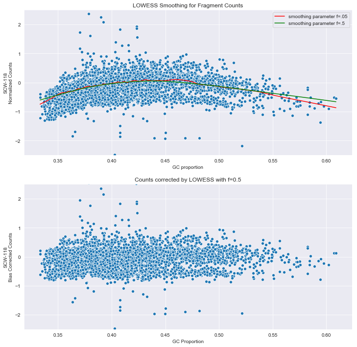
The plots above show how the corrected data looks.

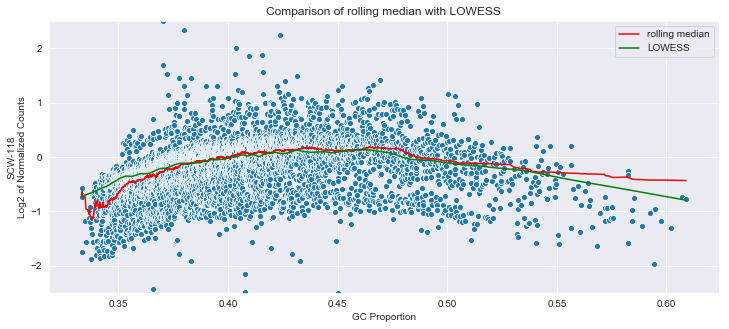
Rolling median and cnvkit

cnvkit uses the rolling median to correct for GC bias. Essentially it takes a window around each GC value, takes the median of the data in that window, and then shifts that to zero. NOTE THAT CNVKIT APPLIES THIS TO THE LOG2 OF THE COUNTS!

import scipy.signal as signal

F=pd.DataFrame([GC['GC'],np.log2(normal[cells].iloc[:,10])])
F=F.transpose()

order=np.argsort(F['GC'])

Y = F.iloc[order,:].copy()
Z=Y.iloc[:,1].rolling(251,min_periods=1).median()
Y.loc[:,'med']=Z
j=sns.scatterplot(Y['GC'],Y.iloc[:,1])
j.set_ylim([-2.5,2.5])
j=sns.lineplot(Y['GC'],Y['med'],ax=j,color='red',label='rolling median')
j=sns.lineplot(B[:,0],B[:,1],color='green',ax=j,label='LOWESS')
j.set_ylabel('SCW-118\nLog2 of Normalized Counts')
j.set_xlabel('GC Proportion')
j.set_title('Comparison of rolling median with LOWESS')
h,l=j.get_legend_handles_labels()
j.legend(h,l)
j.get_figure().set_size_inches(12,5)

j=sns.scatterplot(Y['GC'],Y.iloc[:,1]-Z)
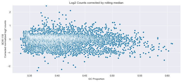
j.set_title('Log2 Counts corrected by rolling median')
j.set_ylabel('SCW-118\n Corrected normalized log2 counts')
j.set_xlabel('GC Proportion')
j.set_ylim([-2.5,2.5])
j.get_figure().set_size_inches(12,5)

Concluding remarks

The two methods give very similar results, and both are quite ad hoc, depending on the choice of smooth parameter (for LOWESS) and window size (for the rolling median).