TSNE annotated
These notes are based on the python implementation of TSNE from van er Maaten’s web page. The goal is to illuminate the algorithm by looking closely at the implementation.
Equation, page, and section references are to the paper Visualizing High-Dimensional Data Using t-SNE, Journal of Machine Learning Research 9(Nov):2579-2605, 2008.
import numpy as np
import pandas as pd
import pylab
Distances between data points as probabilities
The overall input to this implementation is a numpy array $X$ whose $n$ rows are points in $\mathbf{R}^{d}$. The goal is to compute an $n\times 2$ array $Y$ giving the embedding coordinates.
For a fixed point $x_j$, the TSNE algorithm defines “conditional probabilities”
where the variances $\sigma_i^2$ depend on the point $x_i$.
Imagine taking a step in a random walk starting at $x_i$. The underlying idea behind these probabilities is to think of $p_{j|i}$ as the chance that, starting at $x_i$, one would select $x_j$ as the next step. Essentially, points that are equidistant from $x_i$ are equally likely to be chosen, and the chance of selecting $x_j$ drops off like $e^{-r^2/2\sigma_i^2}$ as the distance $r$ between $x_i$ and $x_j$ increases.
Perplexity
In order to choose the $\sigma_i$ appropriately, tsne uses the notion of the perplexity of a probability distribution. To definte the perplexity, recall that the (Shannon) entropy at the point $x_i$ of the (conditional) probability distribution $p_{j|i}$ is The perplexity $\mathrm{perp}$ is the exponential $\mathrm{perp}_i=2^{H_i}$.
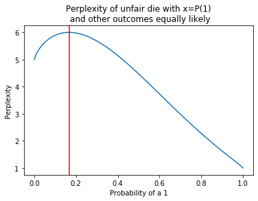
One simple observation is that the perplexity of a uniform distribution on $N$ points is $N$. The plot below considers a die where the chance of rolling a ‘1’ varies between zero and 1, and the chance of rolling anything other than 1 is constant. When the chance of 1 is $1/6$, the overall distribution is uniform and the perplexity is $6$. As the probability concentrates on $1$ the perplexity drops off to 1.
In the tsne setting, the perplexity is a way to measure the “effective number of neighbors” of a point. The algorithm adjusts the variances so that the perplexity at each point is some pre-specified value $\mathbf{perp}$.
In some sense this scales the data so that every point has the same number of neighbors.
from numpy import log2
def perp(p):
L=[p]+[(1-p)/5.0]*5
H=-sum([x*log2(x) for x in L if x!=0])
return 2**H
x=np.linspace(0,1,100)
y=[perp(t) for t in x]
p=pylab.plot(x,y)
t=pylab.title('Perplexity of unfair die with x=P(1)\n and other outcomes equally likely')
pylab.xlabel('Probability of a 1')
pylab.ylabel('Perplexity')
l=pylab.axvline(1/6.0,color='red')
Computing pairwise distances
The tsne implementation uses a nice numpy construction to compute the pairwise distances.
def pdiff(X):
(n,d) = X.shape
# np.square is the elementwise square; axis=1 means sum the rows.
# so sum_X is the vector of the norms of the x_i
sum_X = np.sum(np.square(X),1)
# ||x_i-x_j||^2=||x_i||^2+||x_j||**2-2(x_i,x_j)
# np.dot(X,X.T) has entries (x_i,x_j)
# in position (i,j) you add ||x_i||^2 and ||x_j||^2 from the two sums with the transpose
# the result is that D is a symmetric matrix with the pairwise distances.
D = np.add(np.add(-2*np.dot(X,X.T),sum_X).T,sum_X)
return D
Given the pairwise distances, we can compute the conditional probabilites $p_{j|i}$. The implementation uses the precisions $\beta_i=1/2\sigma_i^2$ instead of the variances. You have to be a bit cautious about the fact that $p_{i|i}=0$.
The function Hbeta in the implementation computes the probabilities and the perplexity
for a single row of the distances matrix with a specified precision $\beta$.
It is called with a row of the distance matrix $D$ with the $i^{th}$ entry deleted.
Let $S_i$ be the denominator of the expression for $p_{j|i}$ .
The entropy is
which gives
def Hbeta(D=np.array([]), beta=1.0):
"""
Compute the perplexity and the P-row for a specific value of the
precision of a Gaussian distribution.  Note that D is the i_th row
of the pairwise distance matrix with the i_th entry deleted.
"""

# Compute P-row and corresponding perplexity
# at this point, P is the numerator of the conditional probabilities
P = np.exp(-D.copy() * beta)
# sumP is the denominator, the normalizing factor
sumP = sum(P)

# the entropy is the sum of p \log p which is P/sumP
# Checking with the formula above, sumP = S_i and np.sum(D*P/sumP) is the dot
# product of the distances with the probabilities

H = np.log(sumP) + beta * np.sum(D * P) / sumP

# now normalize P to be the actual probabilities and return them
P = P / sumP
return H, P
The goal is to adjust the precisions (the $\beta_i$ ) so that the perplexity at each point is the same. The paper argues that the algorithm is robust to changes in this target perplexity, and that it is typically between 5 and 50 – see page 2582. The technique is to do binary search on beta until the perplexity is within tolerance of the goal (or until 50 tries have passed).
def x2p(X=np.array([]), tol=1e-5, perplexity=30.0):
"""
Performs a binary search to get P-values in such a way that each
conditional Gaussian has the same perplexity.
"""

# Initialize some variables
print("Computing pairwise distances...")
(n, d) = X.shape
sum_X = np.sum(np.square(X), 1)
D = np.add(np.add(-2 * np.dot(X, X.T), sum_X).T, sum_X)

P = np.zeros((n, n))
beta = np.ones((n, 1))
logU = np.log(perplexity)

# Loop over all datapoints
for i in range(n):

# Print progress
#if i % 500 == 0:
print("Computing P-values for point %d of %d..." % (i, n))

# prep for binary search on beta

betamin = -np.inf
betamax = np.inf

# Compute the Gaussian kernel and entropy for the current precision
# the first line drops the ith entry in row i from the pairwise distances
# Hbeta in the second line expects this

Di = D[i, np.concatenate((np.r_[0:i], np.r_[i+1:n]))]
(H, thisP) = Hbeta(Di, beta[i])

# Evaluate whether the perplexity is within tolerance
Hdiff = H - logU
tries = 0
while np.abs(Hdiff) > tol and tries < 50:

# If not, increase or decrease precision (via binary search)
if Hdiff > 0:
betamin = beta[i].copy()
if betamax == np.inf or betamax == -np.inf:
beta[i] = beta[i] * 2.
else:
beta[i] = (beta[i] + betamax) / 2.
else:
betamax = beta[i].copy()
if betamin == np.inf or betamin == -np.inf:
beta[i] = beta[i] / 2.
else:
beta[i] = (beta[i] + betamin) / 2.

# Recompute the values
(H, thisP) = Hbeta(Di, beta[i])
Hdiff = H - logU
tries += 1

# Set the final row of P, reinserting the missing spot as 0
P[i, np.concatenate((np.r_[0:i], np.r_[i+1:n]))] = thisP

# Return final P-matrix
# report mean value of sigma, but not the actual sigma values
print("Mean value of sigma: %f" % np.mean(np.sqrt(1 / beta)))
return P
One preliminary step is a linear dimension reduction; here that’s done by a PCA calculation.
def pca(X=np.array([]), no_dims=50):
"""
Runs PCA on the NxD array X in order to reduce its dimensionality to
no_dims dimensions.
"""

print("Preprocessing the data using PCA...")
(n, d) = X.shape

# center the columns, so each column has mean zero
X = X - np.tile(np.mean(X, 0), (n, 1))

# project onto the first no_dims eigenspaces
(l, M) = np.linalg.eig(np.dot(X.T, X))
Y = np.dot(X, M[:, 0:no_dims])
return Y
The basic ingredients of the main algorithm are now the data X, possibly passed through a PCA dimensionality reduction, and then the computed variances so that the perplexities of the conditional distributions at each point are all (roughly) the same. Our goal is to find a set of points Y in (usually) 2 dimensions that capture the relatonships among the X points.
The tsne algorithm symmetrizes the $p_{i|j}$ and $p_{j|i}$ to yield $p_{ij}=(p_{i|j}+p_{j|i})/2$. The paper discusses the logic of this choice compared with, for example, the natural approach of replacing the denominator in the definition of $p_{i|j}$ with the sum over all pairs $k,l$. The point seems to be that if a point is far from all the other points, then the natural approach means that the position of the outlier will have very little effect on the mapped point. The symmetrization technique performs better in this regard. See page 2584.
The points in 2 dimensions also have a conditional distance, but it is given by the student t-kernel instead of the gaussian. That is, Notice that the denominator here is constant, and the probability is symmetric, the so this is a probability that picking two points would yield the pair $y_i$, $y_j$.
The K-L divergence gives a comparison between the $q$ distance on the points $Y$ and the $p$ distance on the $X$ points. where the diagonal elements $p_{ii}=q_{ii}=0$.
The tsne goal is to minimize this K-L divergence by gradient descent.
While perhaps obvious, remember that the KL divergence is a function of the $2n$ variables and so its gradient is a $2n$-vector which is best thought of as an $n\times 2$ matrix where the columns correspond to the derivatives of a single point with respect to the two coordinate directions.
The choice of the t-distribution on the embedded points is a key point, and the paper has the following to say about it (page 2585):
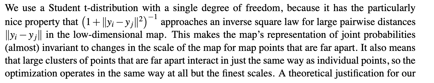
In appendix A of the paper, the authors work out the gradient of the KL divergence (an annoying but straightforward exercise in calculus). The result is that (remembering that $ \partial K/\partial y_{i} $ is a two-dimensional vector)
The code below uses an accelerated gradient descent (gradient descent with momentum). In addition it plays with the learning rate using a version of the “delta-bar-delta” method, which is introduced here.
Another oddity is that the learning rate is set to 500(?).
def tsne(X=np.array([]), no_dims=2, initial_dims=50, perplexity=30.0):
"""
Runs t-SNE on the dataset in the NxD array X to reduce its
dimensionality to no_dims dimensions. The syntaxis of the function is
`Y = tsne.tsne(X, no_dims, perplexity), where X is an NxD NumPy array.
"""

# Check inputs (first thing here looks wrong)
if isinstance(no_dims, float):
print("Error: array X should have type float.")
return -1
if round(no_dims) != no_dims:
print("Error: number of dimensions should be an integer.")
return -1

# Initialize variables
# use eigh and then you don't need the real
X = pca(X, initial_dims).real
(n, d) = X.shape
max_iter = 5000
initial_momentum = 0.5
final_momentum = 0.8
eta = 500
min_gain = 0.01


# initial Y placements are random points in (usually) 2-space
Y = np.random.randn(n, no_dims)
dY = np.zeros((n, no_dims))
iY = np.zeros((n, no_dims))
gains = np.ones((n, no_dims))
Ysave = Y.copy()
Csave = 0.0


# Compute P-values
P = x2p(X, 1e-5, perplexity)
# symmetrize the probabilities; see page 2584.  This makes sure that if a point is far from
# all the other points, its position is still relevant.
P = P + np.transpose(P)
P = P / np.sum(P)

# not clearly documented in the paper but seems to help with convergence
P = P * 4.   # early exaggeration
# avoid zeros
P = np.maximum(P, 1e-12)

# Run iterations
for iter in range(max_iter):

# Compute pairwise affinities using the student t-kernel (equation 4)
sum_Y = np.sum(np.square(Y), 1)
num = -2. * np.dot(Y, Y.T)
num = 1. / (1. + np.add(np.add(num, sum_Y).T, sum_Y))
num[range(n), range(n)] = 0.
Q = num / np.sum(num)
Q = np.maximum(Q, 1e-12)

# Compute gradient

# PQ is a symmetric n x n matrix with entries p_ij-q_ij
PQ = P - Q

# This is a clever way to compute the gradient; dY is n x 2 matrix, each column is a dy_i
for i in range(n):
dY[i, :] = np.sum(np.tile(PQ[:, i] * num[:, i], (no_dims, 1)).T * (Y[i, :] - Y), 0)

# Perform the update
if iter < 20:
momentum = initial_momentum
else:
momentum = final_momentum

# this business with "gains" is the bar-delta-bar heuristic to accelerate gradient descent
# code could be simplified by just omitting it

gains = (gains + 0.2) * ((dY > 0.) != (iY > 0.)) + \
(gains * 0.8) * ((dY > 0.) == (iY > 0.))
gains[gains < min_gain] = min_gain

# this is the momentum update

iY = momentum * iY - eta * (gains * dY)
Y = Y + iY

# recentering the data (doesn't affect the distances between points)
Y = Y - np.tile(np.mean(Y, 0), (n, 1))

#Compute current value of cost function
if (iter + 1) % 100 == 0:
Ysave = np.concatenate([Ysave, Y])
C = np.sum(P * np.log(P / Q))
#print("Iteration %d: error is %f" % (iter + 1, C))
if np.abs(Csave - C)<.001:
break
Csave = C


# Stop lying about P-values
# this is "early exaggeration" which is not really explained in the paper

if iter == 100:
P = P / 4.


# Return solution
return Y, Ysave
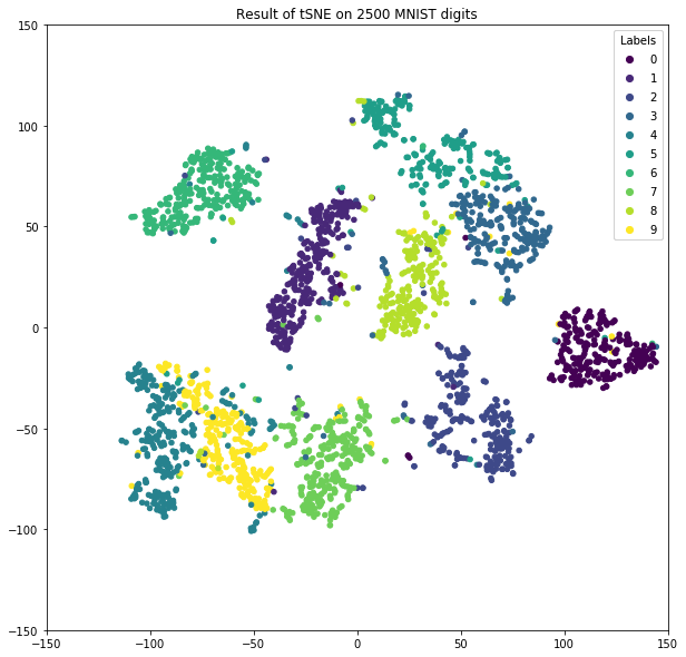
X = np.loadtxt("data/mnist2500_X.txt")
labels = np.loadtxt("data/mnist2500_labels.txt")
# tsne function modified to save status every 100 iterations
Y, Ysave = tsne(X, 2, 50, 20.0)

# save the evolution of the data for graphics later.
np.savetxt("data/tsne_evolution.txt", Ysave, delimiter='\t')
Preprocessing the data using PCA… Computing pairwise distances… Mean value of sigma: 2.386597 Iteration 100: error is 16.072850 Iteration 200: error is 1.382539 Iteration 300: error is 1.184231 Iteration 400: error is 1.113216 Iteration 500: error is 1.078388 Iteration 600: error is 1.057110 Iteration 700: error is 1.043093 Iteration 800: error is 1.033235 Iteration 900: error is 1.026040 Iteration 1000: error is 1.020572 Iteration 1100: error is 1.016277 Iteration 1200: error is 1.012674 Iteration 1300: error is 1.009772 Iteration 1400: error is 1.007440 Iteration 1500: error is 1.005449 Iteration 1600: error is 1.003723 Iteration 1700: error is 1.002224 Iteration 1800: error is 1.000906 Iteration 1900: error is 0.999729 Iteration 2000: error is 0.997927 Iteration 2100: error is 0.997097
Plot of final results.
fig,ax = plt.subplots(1)
scatter=ax.scatter(Y[:, 0], Y[:, 1], 20, c=labels)
ax.get_figure().set_size_inches(10,10)
l = ax.legend(*scatter.legend_elements(),
loc="upper right", title="Labels")
j=ax.add_artist(l)
t=ax.set_title('Result of tSNE on 2500 MNIST digits')
t=ax.set_xlim([-150,150])
t=ax.set_ylim([-150,150])