Genotyping from sequence data

5 minute read

Genotyping from sequence data

These are some notes on the (old) paper:

Li, H. A statistical framework for SNP calling, mutation discovery, association mapping and population genetical parameter estimation from sequencing data. Bioinformatics, Vol. 27, no. 21, 2011, pp. 2987-2993.

For simplicity, we assume we have a diploid individual. We imagine that we do some sequencing experiments on a population in Hardy-Weinberg equilibrium (HWE). We are interested in a particular site in the genome, where we assume that our sequencing experiments yield either a reference allele R or an alternative allele A. We would like to estimate the frequency $\psi$ of the reference allele in the population.

A given individual can have one of three genotypes: RR, RA, and AA. Since the population is in HWE, the frequencies of these genotypes are $\psi^2$, $2\psi(1-\psi)$, and $(1-\psi)^2$.

A sequencing experiment of depth $k$ on an individual yields $l$ reference bases $R_1,\ldots, R_{l}$ and $k-l$ alternative bases $A_{l+1}, \ldots, A_{k}$. Each base also has an associated error $\epsilon_j$ which is the probability that the $j^{th}$ base read is incorrect.

Let $g$ be the number of reference bases in the genotype (so $g=0,1,2$). The likelihood of obtaining $l$ reference bases out of $k$ tries assuming genotype $g=0$ is $P(l|g=0)=\prod_{j=1}^{l}P(\mathrm{read}_j=R|\mathrm{truth}_j=A) \prod_{j=l+1}^{k}P(\mathrm{read}_j=A|\mathrm{truth}_j=A)=\prod_{j=1}^{l}\epsilon_{j}\prod_{j=l+1}^{k}(1-\epsilon_{j})$

In the $g=1$ case, we use the fact that $P(\mathrm{truth}=A)=P(\mathrm{truth}=R)=\frac{1}{2}$ and $P(\mathrm{read}=R|\mathrm{truth}=A)=P(\mathrm{read}=A|\mathrm{truth}=R)=\epsilon$ to conclude that $P(\mathrm{read}=R)=P(\mathrm{read}=R|\mathrm{truth}=R)P(\mathrm{truth}=R)+P(\mathrm{read}=R|\mathrm{truth}=A)P(\mathrm{truth}=A)=\frac{1}{2}$ and similarly $P(\mathrm{read}=A)=\frac{1}{2}.$

Therefore: $P(l|g=1)=\prod_{j=1}^{l}P(\mathrm{read}_j=R)\prod_{j=l+1}^{k}P(\mathrm{read}_j=A)=\frac{1}{2^k}$

Lastly, the computation for $g=2$ is just like the case for $g=0$ and yields $P(l|g=2)=\prod_{j=1}^{l}(1-\epsilon_{j})\prod_{j=l+1}^{k}\epsilon_{j}$

Multiple samples

The calculation above examines the case of what we expect if we do a sequencing experiment on a single individual and attempt to reconstruct the genotype of that individual. But we are interested in the allele frequency in the population. So we do the sequencing experiment on multiple individuals; let $(l_i, k_i)$, for $i=1,\ldots, n$ be the number of reference alleles and the depth that we obtain from experiment $i$. Using the HWE, we have

$P((l_i,k_i)|\psi)=\sum_{g=0}^{2} P((l_i,k_i)|g)P(g|\psi)$ and the combined probability is $P(\{(l_i,k_i)\}_{i=1}^{n}|\psi)=\prod_{i=1}^{n}P((l_i,k_i)|\psi).$

Using this one can, for example, compute the maximum likelihood estimate of $\psi$ by applying the Expectation Maximization algorithm.

The EM algorithm

The EM algorithm proceeds iteratively. First, we assume that we have an initial guess for $\psi$ and treat $\psi$ as a fixed parameter. Given $\psi$ and the data, we find the expected genotype. We write $P_{\psi}$ to remind us that we are treating $\psi$ as fixed for now. Using Bayes Rule we have:

$P_{\psi}(g|d) = \frac{P_{\psi}(d|g)P_{\psi}(g)}{\sum_{g=0}^{2} P_{\psi}(d|g)P_{\psi}(g)}$

Therefore, for a given individual dataset, the expected genotype is

$E(g|d)=\sum_{g=0}^{2}gP_{\psi}(g|d)=\frac{\sum_{g=0}^{2} gP_{\psi}(d|g)P_{\psi}(g)}{\sum_{g=0}^{2} P_{\psi}(d|g)P_{\psi}(g)}$

and the expected genotype for the entire sample is

$E=\frac{1}{n}\sum_{i=1}^{n} E(g|d_i).$

For the maximization step of the EM algorithm, we need to take the maximum likelihood estimate of $\psi$ based on this $E$. But that’s easy, because if the mean genotype is $g$, then the mean number of reference alleles is $g$ and so the reference allele frequency is $g/2$.

The following functions give a crude implementation of the EM algorithm in the paper.

N is the depth (assumed the same for all samples)
r is the number of reference alleles observed in the sample
e is the error probability (assumed the same for all samples)
g is the genotype (0,1,2) – ploidy fixed at 2

import numpy as np
from scipy.special import binom
import matplotlib.pyplot as plt

def p(r,N,g,e):
if g==0:
return binom(N,r)*(e)**r*(1-e)**(N-r)
if g==1:
return binom(N,r)*2**(-N)
if g==2:
return binom(N,r)*(1-e)**r*e**(N-r)

def L(r,N,g,e,psi):
'''
r - observed number of reference alleles in the sample
N - depth
g - genotype
e - error rate (asumed the same for all reads)
psi - reference allele frequency

Returns: P((r,N)|g, \psi)
'''
return p(r,N,g,e)*binom(2,g)*(psi**g*(1-psi)**(2-g))

def mpsinew1(r,N,e,psi):
'''
r - observed number of reference alleles
N - depth
e - error rate
psi - reference allele frequency

Returns: Expected genotype E(g|d,psi)
'''
return np.sum([g*L(r,N,g,e,psi) for g in [0,1,2]])/np.sum([L(r,N,g,e,psi) for g in [0,1,2]])


def EM(N,e,psi0,D,iters):
'''
N - depth
e - error rate
psi0 - initial guess for allele frequency in the population
D - the data (a list of integers between 0 and N)
iters - the number of iterations

Returns: list of iters new estimates for psi
'''
psi=psi0
ans = []
for i in range(iters):
S=[mpsinew1(r,N,e,psi) for r in D]
psi=np.sum(S)/2/len(D)
ans.append(psi)
return ans

N=20
e=.1
psi0=.5
D=[13,15,12,13,17]
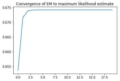
L=EM(N,e,psi0,D,20)
a=plt.plot(range(len(L)),L)
t=plt.title('Convergence of EM to maximum likelihood estimate')

Bayesian perspective

From a Bayesian point of view, we have a hierarchical model where we can pick:

a uniform prior on $\psi$ (for example)
the genotype is distributed as $\mathrm{binomial}(2,\psi)$
given the genotype, and assuming constant depth $N$ and constant error rate $\epsilon$, the number $r$ of reference alleles is distributed as
$\mathrm{binomial}(N,1-\epsilon)$ if $g=2$
$\mathrm{binomial}(N,1/2)$ if $g=1$
$\mathrm{binomial}(N,\epsilon)$ if $g=0$.

We can cast this into the STAN language and use its NUTS sampler to get a distribution for $\psi$.

import pystan

genotype_code = """
data {
int<lower=0> N ; // sequencing depth
real e ; //error probability
int<lower=0> S ; // number of samples
int r[S]; // number of reference alleles in each sample
}
parameters {
real psi;  // reference allele frequency

}
model {
real a ;

for (i in 1:S){
a=0 ;
for (j in 0:2) {
a += exp(binomial_lpmf(r[i] | N, .5*((2-j)*e + j*(1-e)))+binomial_lpmf(j | 2,psi)) ; // sum over the genotypes
}
target += log(a) ; // sum over the samples to get likelihood of the data
}
}
"""

sm=pystan.StanModel(model_code=genotype_code)

We make some sample data assuming that the reference allele frequency is .7 and there’s some variation around the expected number.

from scipy.stats import binom, randint
def r(i):
if i==0:
return randint(0,2).rvs(1)[0]
if i==1:
return randint(-1,2).rvs(1)[0]
if i==2:
return randint(-1,1).rvs(1)[0]
X = binom(2,.7).rvs(1000)
Y = 10*X+np.array([r(X[i]) for i in range(1000)])
genotype_data={'N':20,'e':.2,'S':1000, 'r':Y}
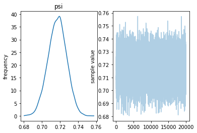
genotype_fit = sm.sampling(data=genotype_data,iter=10000,chains=4)
genotype_fit

Inference for Stan model: anon_model_601a00380873c2229319e991f2f183a0. 4 chains, each with iter=10000; warmup=5000; thin=1; post-warmup draws per chain=5000, total post-warmup draws=20000.

mean se_mean sd 2.5% 25% 50% 75% 97.5% n_eff Rhat psi 0.72 1.2e-4 0.01 0.7 0.71 0.72 0.72 0.74 7389 1.0 lp__ -3822 7.2e-3 0.69 -3824 -3822 -3822 -3822 -3822 9101 1.0

Samples were drawn using NUTS at Wed May 1 14:53:04 2019. For each parameter, n_eff is a crude measure of effective sample size, and Rhat is the potential scale reduction factor on split chains (at convergence, Rhat=1).

fig=genotype_fit.plot()

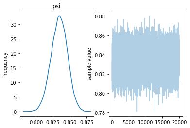
Now we use the same data, but with a higher error probability. The effect seems to be to shift the distribution of $\psi$ to the right.

genotype_data={'N':20,'e':.4,'S':1000, 'r':Y}
genotype_fit = sm.sampling(data=genotype_data,iter=10000,chains=4)
genotype_fit

Inference for Stan model: anon_model_601a00380873c2229319e991f2f183a0. 4 chains, each with iter=10000; warmup=5000; thin=1; post-warmup draws per chain=5000, total post-warmup draws=20000.

mean se_mean sd 2.5% 25% 50% 75% 97.5% n_eff Rhat psi 0.83 1.4e-4 0.01 0.81 0.83 0.83 0.84 0.86 7373 1.0 lp__ -6583 7.3e-3 0.71 -6585 -6583 -6583 -6583 -6583 9291 1.0

Samples were drawn using NUTS at Wed May 1 14:38:22 2019. For each parameter, n_eff is a crude measure of effective sample size, and Rhat is the potential scale reduction factor on split chains (at convergence, Rhat=1).

fig=genotype_fit.plot()

Jeremy Teitelbaum

Genotyping from sequence data