Amplification Bias

See Calibrating genomic and allelic coverage bias in single-cell sequencing by Zhang, et. al.

To obtain enough material to sequence single cells, one must amplify a tiny amount of DNA many times over. There are a number of methods for doing this, and each of them introduces a different type of bias into the process. A standard approach used for single-cell DNA is called MDA (multi-strand displacement amplification) – other methods are PCR and MALBAC. Understanding how these methods work is another project, but for the purposes of this discussion the key feature is the length scale on which they operate. If the pieces of amplified DNA (called amplicons) have a characteristic length, then this will introduce a correlation structure into the sequences because pieces of the genome within that length scale are more likely to be covered. The Zhang paper examines this autocorrelation structure by comparing single cell sequencing with bulk sequencing at various depths. They find that, for single cells, the coverage depth shows autocorrelation on a length scale of ~100kb that is absent from the bulk sequences. This reflects the amplification bias.

One important feature of this ‘amplicon-scale’ auto-correlation is that it doesn’t decay with increasing sequencing depth. This is because this bias is introduced BEFORE the DNA is broken into fragments and sequenced. Higher depth sequencing gives a better picture of the amplified DNA, not of the original DNA.

Let’s illustrate this with a simulation. The relevant parameters are:

• The length of the chromosome N
• The length of the amplicons L
• The amplicon coverage = (Number of Amplicons)(L/N)
• The read length r
• The read coverage = (Number of reads)(r/N)

We generate the read coverage in two steps. First, we choose the amplicon locations at random and compute the coverage of each base by an amplicon. Since the reads are chosen from the amplicons, not the original sequences, the probability of a read starting at a particular base is then the amplicon coverage of that base divided by the length of the chromosome – up to normalization.

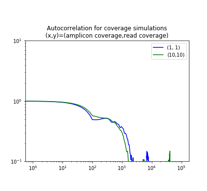
The figure below shows the autocorrelation for two simulated samples, one where the amplicons have 10-fold coverage of the genome ãnd the reads also give 10-fold coverage; and one where the coverage is 1-fold in each case. Note that the graphs show the kink around the read length and then are constant until the amplicon length.

Simulation	Figure 2a from Zhang, et. al.

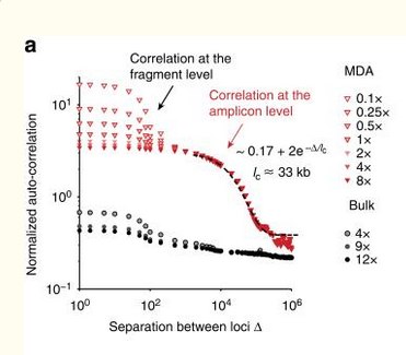The two plots use different normalizations for the autocorrelation, but they show the same qualitative properties.

Here is the code for this.

import numpy as np
from statsmodels.tsa.stattools import acf
import matplotlib.pyplot as plt

def sim(N, amplicon_length, amplicon_coverage, read_len, read_coverage):
H=np.zeros(N)
G=np.zeros(N)
num_amplicons = N*amplicon_coverage//amplicon_length
X=np.random.randint(N,size=num_amplicons)
U=np.ones(amplicon_length)
# compute the coverage of the genome by amplicons
for i in X:
e=np.min([N-i,amplicon_length])
H[i:(i+e)]=H[i:(i+e)]+U[:e]
num_reads = N*read_coverage//read_len
Y=np.random.choice(N,size=num_reads,p=H/H.mean()/N)
U=np.ones(read_len)
for i in Y:
e=np.min([N-i,read_len])
G[i:(i+e)]=G[i:(i+e)]+U[:e]
return G

# 100000 base pairs; amplicon length 2000; read length 100
# compare coverages: amplicon 1, read 1 vs amplicon 10, read 10

G_1_1=sim(100000,2000,1,100,1)
G_10_10=sim(100000,2000,10,100,10)

# Draw a picture
fig = plt.figure()
fig.set_size_inches(6,10)
ax = fig.add_subplot(2,1,1)
AC1=acf(G_1_point1,nlags=N)
AC2=acf(G_10_10,nlags=N)
line, = ax.plot(AC1,color='blue',label=(1,1))
line2=ax.plot(AC2,color='green',label=(10,10))
ax.set_title('Autocorrelation for coverage simulations\n (x,y)=(amplicon coverage,read coverage))
ax.set_ylim([.1,10])
ax.set_xscale('log')
ax.set_yscale('log')
t=ax.legend()