6 Gradient Descent
6.1 Introduction
A common mathematical theme throughout machine learning is the problem of finding the minimum or maximum value of a function. For example, in linear regression, we find the “best-fitting” linear function by identifying the parameters that minimize the mean squared error. In principal component analysis, we try to identify the scores which have the greatest variation for the given set of data, and for this we needed to maximize a function using Lagrange multipliers. In later lectures, we will see many more examples where we construct the “best” function for a particular task by minimizing some kind of error between our constructed function and the true observed values.
In our discussion of PCA and linear regression, we were able to give analytic formulae for the solution to our problems. These solutions involved (in the case of linear regression) inverting a matrix, and in the case of PCA, finding eigenvalues and eigenvectors. These are elegant mathematical results, but at that time we left open the question of how to actually compute these quantities of interest in an efficient way. In this section, we will discuss the technique known as gradient descent, which is perhaps the simplest approach to minimizing a function using calculus, and which is at the foundation of many practical machine learning algorithms.
6.2 The Key Idea
Suppose that we have a function \(f(x_1,\ldots, x_{k})\) and we wish to find its minimum value. In Calculus classes, we are taught to take the derivatives of the function and set them equal to zero, but for anything other than the simplest functions this problem is not solvable in practice. In real life, we use iterative methods to find the minimum of the function \(f\).
The main tool in this approach is the gradient of a function. Recall from multivariable calculus that, given a function \(f(x_1,\ldots, x_{k})\), the gradient \(\nabla f\) of \(f\) is the vector made up of the partial derivatives of \(f\):
\[ \nabla f = \begin{bmatrix} \frac{\partial f}{\partial x_{1}} \\\vdots \\ \frac{\partial f}{\partial x_{k}}\end{bmatrix} \tag{6.1}\]
The gradient \(\nabla f\) is an example of a vector field. It is a vector whose entries are functions. If we evaluate those functions at a point \(x\), we obtain a vector \((\nabla f)(x)\).
We can think of a vector field as a way to attach a vector \((\nabla f)(x)\) to each point \(x\in\mathbf{R}^{k}\).
Proposition: Let \(f(x_1,\ldots, x_{k})\) be a function and let \(\nabla f\) be its gradient. Then at each point \(x\) in \(\R^{k}\), the gradient \((\nabla f)(x)\) is a vector that points in the direction in which \(f\) is increasing most rapidly from \(x\) and \((-\nabla f)(x)\) points in the direction in which it decreases most rapidly. If \((\nabla f)(x)=0\), then \(x\) is a critical point of \(f\).
This fact arises from thinking about the directional derivative of a function.
The directional derivative \(D_{v}f\) measures the rate of change of \(f\) as one moves with velocity vector \(v\) from a chosen point \(a\in\mathbf{R}^{k}\) and it is defined as \[
D_{v}f(a) = \frac{d}{dt}f(a+tv)|_{t=0}
\]
If \(a=(a_1,\ldots, a_{k})\) and \(v=(v_{1},\ldots, v_{k})\), then \[ f(a+tv) = f(a_{1}+tv_{1},\ldots, a_{k}+tv_{k}). \] Since \[ \frac{d}{dt}(a_{i}+tv_{i})=v_{i} \] we can compute from the chain rule that \[ D_{v}f(a) = \sum_{i=1}^{k} \frac{\partial f}{\partial x_{i}}(a)v_{i} = (\nabla f)(a)\cdot v \] where \(\nabla f\) is the gradient of \(f\) as in Equation 6.1.
If we travel from a point \(a\) with velocity vector \(v\), the rate of change of \(f\) along our path will depend on how fast we travel as well as the direction we choose. In other words, \(D_{v}f\) depends on the magnitude of \(v\), as well as its direction. To remove this dependence on the magnitude of \(v\), we scale \(v\) to be a unit vector.
Now \[ (\nabla f)(a)\cdot v=\|(\nabla f)(a)\|\|v\|\cos\theta=\|(\nabla f)(a)\|\cos \theta \] where \(\theta\) is the angle between \(v\) and \((\nabla f)(a)\). Clearly this dot product is maximized when \(v\) is parallel to \((\nabla f)(a)\) so \(\cos\theta=1\). If \(v\) is opposite to \((\nabla f)(a)\), then \(\cos\theta=-1\) and the dot product is minimized.
6.3 The Algorithm
To exploit the fact that the gradient points in the direction of most rapid increase of our function \(f\), we adopt the following strategy. Starting from a point \(x\), compute the gradient \((\nabla f)(x)\) of \(f\). Take a small step in the direction of the gradient – that should increase the value of \(f\). Then do it again, and again; each time, you move in the direction of increasing \(f\), but at some point the gradient becomes very small and you stop moving much. At that moment, you stop. You have reached the highest value of \(f\) in the immediate vicinity. This is called “gradient ascent” to a local maximum.
If we want to minimize, not maximize, our function, then we want to move opposite to the gradient in small steps. This is the more common formulation.
6.3.1 Gradient Descent Algorithm
Given a function \(f:\mathbb{R}^{k}\to \mathbb{R}\), to find a point where it is minimized, choose:
- a starting point \(c^{(0)}\),
- a small constant \(\nu\) (called the learning rate)
- and a small constant \(\epsilon\) (the tolerance).
Iteratively compute \[ c^{(n+1)}=c^{(n)} -\nu(\nabla f)(c^{(n)}) \] until \(\|c^{(n+1)}-c^{(n)}\|<\epsilon\).
Then \(c^{(n+1)}\) is an (approximate) critical point of \(f\).

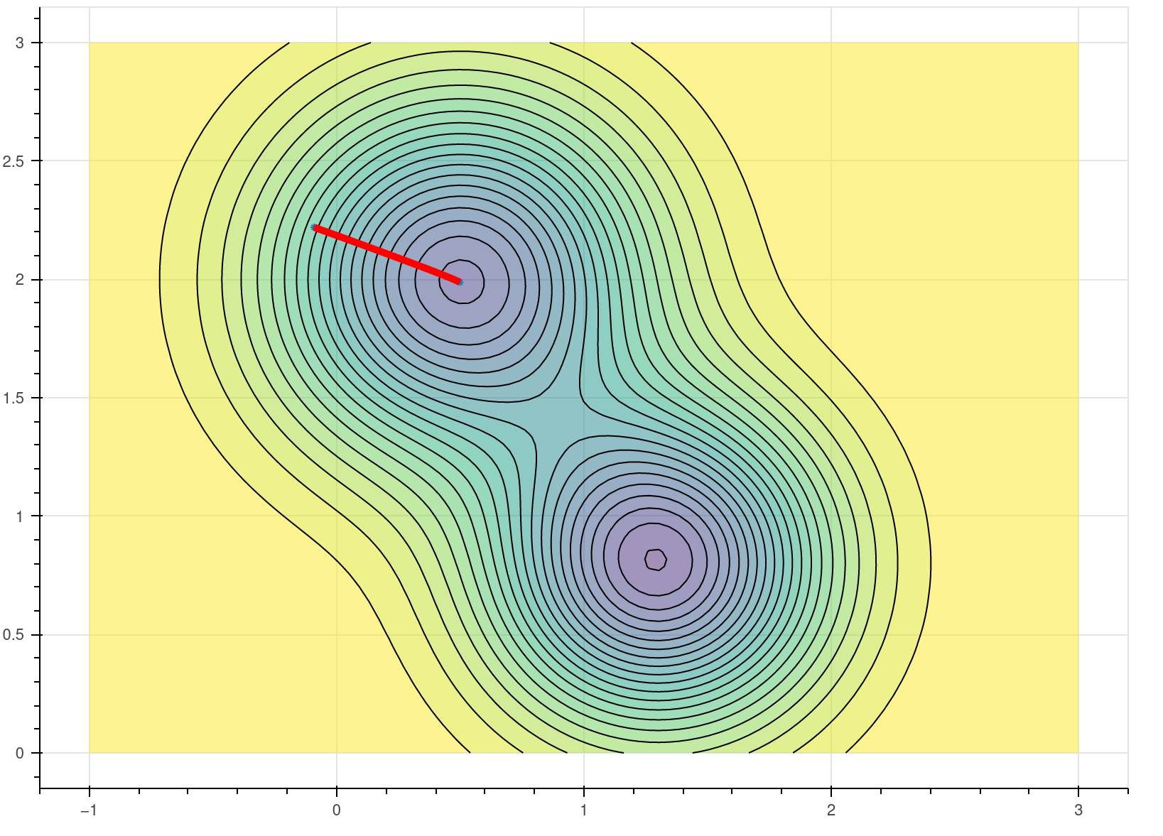
The behavior of gradient descent, at least when all goes well, is illustrated in Figure 6.1 for the function \[ f(x,y) = 1.3e^{-2.5((x-1.3)^2+(y-0.8)^2)}-1.2e^{-2((x-1.8)^2+(y-1.3)^2)}. \]
Figure 6.1 is a contour plot, with the black lines at constant height and the colors indicating the height of the function. This function has two “pits” or “wells” indicated by the darker, “cooler” colored regions. The red line shows the gradient descent algorithm heading “downhill” towards a nearby local minimum.
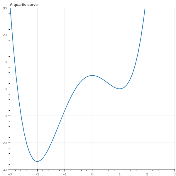
To get a little more perspective on gradient descent, consider the one-dimensional case, with \[ f(x)=3x^4+4x^3-12x^2+5. \] This is a quartic polynomial whose graph has two local minima and a local maximum, depicted in Figure 6.2.

In this case the gradient is just the derivative \[ f'(x)=12x^3+12x^2-24x \] and the iteration is \[ c^{(n+1)} = c^{(n)}-12\nu((c^{(n)})^3+(c^{(n)})^2-2c^{(n)}). \]
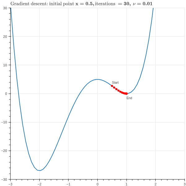
From this simple example we can see the power and also the pitfalls of this method. Suppose we choose \(c^{(0)}=.5\), \(\nu=.01\), and do \(30\) iterations of the main loop in our algorithm. The result is shown in Figure 6.3 .

As we hope, the red dots quickly descend to the bottom of the “valley” at the point \(x=1\). However, this valley is only a local minimum of the function; the true minimum is at \(x=-2\). Gradient descent can’t see that far away point and so we don’t find the true minimum of the function. One way to handle this is to run gradient descent multiple times with random starting coordinates and then look for the minimum value it finds among all of these tries.
6.4 Linear Regression via Gradient Descent
In our discussion of Linear Regression in Chapter 1, we used Calculus to find the values of the parameters that minimized the squared difference between the predicted and desired values. If our features were stored in the matrix \(X\) (with an additional column of \(1\)’s) and our target values in the vector \(Y\), then we showed that the optimal parameters \(M\) were given by
\[ M=D^{-1}X^{\intercal}Y \]
where \(D=X^{\intercal}X\). This set of parameters minimizes the squared error:
\[ L = \| Y-XM \|^2. \]
See Equation 1.7 and Equation 1.8.
One problem with this approach is the need to invert the matrix \(D\), which is a serious computation in its own right. We can avoid relying on matrix inversion by approaching this problem numerically via gradient descent, using the computation of the gradient in Equation 1.5:
\[ \nabla E = \left[\begin{matrix} \frac{\partial}{\partial M_1}L \\ \frac{\partial}{\partial M_2}L \\ \vdots \\ \frac{\partial}{\partial M_{k+1}}L\end{matrix}\right] = -2 X^{\intercal}Y + 2 X^{\intercal}XM \]
The gradient descent algorithm looks like this.
6.4.1 Gradient Descent Algorithm for Linear Regression
Set \(M^{(0)}\) to a random vector in \(\R^{k+1}\) for an initial guess and choose a learning rate parameter \(\nu\). Compute \(A=X^{\intercal}Y\) (an element of \(\R^{k+1}\)) and \(D=X^{\intercal}X\) (a \((k+1)\times (k+1)\) matrix).
Iteratively compute
\[ M^{(j+1)}=M^{(j)}-\nu(-2A+2DM^{(j)}) \]
until a stopping condition is met. For example, stop if:
- the squared error \(\|Y-XM^{(j)}\|^2\) is sufficiently small, or
- the squared error decreases by less than some tolerance on each iteration, or
- the entries of \(M^{(j)}\) change by less than some tolerance.
Notice that this algorithm does not need computation of \(D^{-1}\).
6.5 Stochastic Gradient Descent
Using the numerical approach to linear regression avoids inverting the matrix \(D=X^{\intercal}X\), but still leaves us the task of computing it. Typically \(X\) has many rows, and so this computation is time-intensive. We would like to avoid having to use all of the data for each iteration of our algorithm.
Stochastic gradient descent is a method for numerical optimization that does not require use of all the data on each iteration. Instead, it uses each data point sequentially. Let’s look at this in the context of linear regression. Suppose we have an estimate \(M\) for the parameters. We take one data point \(x\) — a single row of the data matrix \(X\) — and the associated target value \(y\). The error for this particular point is \((y-xM)^2.\)
The gradient of the squared error (SE), viewed as a function of the weights \(M\), at this particular point is
\[ \nabla SE = -2x^{\intercal}(y-xM) \]
Notice that \(y-xM\) is just a scalar, so this is a scalar multiple of the vector \(x\).
Now we iterate over the data, adjusting the parameters \(M\) by this per-sample gradient. Each pass through the entire set is sometimes called an “epoch.”
6.5.1 Stochastic Gradient Descent for Linear Regression
Set \(M^{(0)}\) to a random starting vector in \(\R^{k+1}\) and choose a learning rate parameter \(\nu\).
For each sample \((x_{i},y_{i})\) consisting of a row of the data matrix \(X\) and its corresponding target value, adjust the parameters by the gradient of the error associated with this point:
\[ M^{(j+1)} = M^{(j)}-\nu(-2x_i^{\intercal} (y_i-x_iM^{(j)})) = M^{(j)}+2\nu x_i^{\intercal}(y_i-x_iM^{(j)}) \]
Here \(x_{i}^{\intercal}\) and \(M^{(j)}\) are column vectors and \(y_i-x_iM^{(j)}\) is a scalar.
Run through the data set multiple times and track the error \((y_i-x_iM^{(j)}S)^2\) for each pair \((x_i,y_i)\).
These errors will bounce around but trend overall downward. When the error becomes smaller than a threshold, or when the difference between successive errors becomes smaller than a threshold, stop.
Note: To minimize the bias introduced by the particular order in which you process the data, it’s often worthwhile to shuffle the order in which you consider the points \((x,y)\) in each epoch.